 X9i: How to Achieve a Maximum
Performance?
X9i: How to Achieve a Maximum
Performance?

… … … This compendium
is big (±15MB), please take
your time while it is downloading ... … …
WARNING: Some people
report once in a while an error while downloading in IE.
Firefox (http://www.mozilla.com/firefox/ ) works fine.
To ease the navigation and browsing through
this compendium, a clickable Table of
Contents in a separate frame is provided in this temporary link.
Fora on SUUNTO X9i:
□
Yahoo
WriststopTrainers forum: http://health.groups.yahoo.com/group/WriststopTrainers/ . Only in this forum I reply on
questions concerning this compendium.
□
‘X9i
User’s Group’ and the ‘Cross Forum’ in SuuntoSports: http://suuntosports.com/Default.asp
Table of contents
2 Birds eye view of the features of the X9i trekking wristop
3.2.1 X9i user interface and DISPLAY MODES
3.2.2 Setting up the displayed GPS UNITS
3.2.2.1 Available datums and position notations in X9i
3.2.2.2 How to set correctly the datum and position format in
X9i?
3.2.2.2.2 Correct assignment procedure
3.2.2.3 An example showing the assignment procedure
3.2.3 Setting up the current time
3.2.4 Setting up the X9i with STM
4 Recording Tracks, ALTitude, MEMory points and other data
4.1 Recording Tracks and ALTitude
4.1.1 Accurate position recording
4.1.1.1 Start a track log AFTER the
ACTIVITY is set to ►
4.1.1.2 Continue a track log NOT by setting the GPS ‘on’
4.1.1.3 GPSFIX, recording intervals, memory capacity, battery lifetime
4.1.2 Accurate altitude recording
4.1.2.1 Influences on altitude measurement: barometric drift
and ISA
4.1.2.2 Guidelines to obtain very accurate estimations of the
altitude
4.1.2.3 Altitude measurements at the same spot
4.1.2.4 A few practical examples
4.1.2.4.1 Example 1: Pic de Moufons
4.1.2.5 Conclusions on ISA corrections
4.3 Instant display of the recorded data
5.1 Digital mapping software with X9i drivers
5.1.1 Displaying Tracks in CompeGPS
5.1.1.1 Setting up CompeGPS LAND
5.1.1.2 Reading Tracks / Routes / Waypoints
5.1.1.3 Mapping in CompeGPS: OPTION 1: Internet servers.
5.1.1.4 Mapping in CompeGPS: OPTION 2: Digital maps.
5.1.1.5 Mapping in CompeGPS: OPTION 3: Scanned maps
5.1.1.6 Putting things together in 3D
5.1.2 Displaying Tracks in STM (Suunto Track Manager)
5.1.2.1 Setting up X9i with STM
5.1.2.2 Calibrating a scanned map, and displaying maps
5.1.2.3 Reading and displaying Tracks, Waypoints, Routes
5.2 Digital mapping software without X9i drivers
5.2.1 Displaying in other software than Google Earth
5.2.1.1 Example: Transcode track logs with GPSBabel to NGI
Digital Topographic Maps
5.2.2 Displaying in GoogleEarth
5.2.2.1 Transcoding to GoogleEarth with GPSVisualizer
5.2.2.2 Transcoding to GoogleEarth with
STE (Suunto Track Exporter)
5.3 What to do with Google tracks ?
6.1 Digital mapping software with X9i drivers.
6.1.1 Programming Routes / Individual Waypoints in COMPEGPS
6.1.1.1 Creating a ROUTE/WAYPOINT
6.1.1.2 Writing the Route to X9i
6.1.2 Programming Routes / Individual Waypoints in STM
6.1.2.1 Creating a Route from scratch
6.1.2.2 Editing/Inserting/Deleting a Waypoint somewhere in the
route
6.1.2.3 Splitting the Route into pieces
6.1.2.4 Concatenate two Routes together
6.2 Digital mapping software without X9i drivers
6.3 Direct programming on the X9i display
6.3.1 Be careful about the map DATUM and Grid
8 Position accuracy of the X9i
8.2 Three illustrative examples
8.2.2 A less demanding example
8.2.3 A best practice example for demanding conditions
8.3 Which distance is the most accurate one?
9.3 Which battery pack is the best?
9.4 Effects of degraded charging
9.5 Alternatives; but watch out.
10 Using X9i in real life: how to make things work
10.1 Preparation of the hike: creation of the route
11.1 Firmware bugs, abnormal behavior in X9i
11.2 Weak points of X9i and related best practices
11.3 Bugs and weak points in STM + workarounds
12 APPENDIX: Cartography and GPS in a nutshell
12.1 datums and position coordinate systems
12.1.1 Orthometric and ellipsoidal height
12.1.2 Geographic and square coordinates
12.3 Do certain UTM coordinates refer always to the same location on earth?
15 Document printing instructions
This document does not explain the
weaknesses (bugs, weird effects) and strengths of the X9i and accompanying
Suunto Trek Manager ‘alone’. It reports
as well on how you can get the maximum out of this tiny wristop GPS navigator.
This is done by discussing how to use the X9i from the very first beginning,
how to avoid bootstraps, and how to integrate the X9i intelligently with other
valuable softwares.
The document is set up in the same
chronological order as you would use the X9i and accompanying softwares:
1. First you would like to set up the
X9i ( Chapter 3) to record a first track log (Chapter 4);
2. Then you would like to display that
first track log onto a digitized map or in digital mapping software (Chapter 5);
3. The next logical step is to program
a WAYPOINT or a ROUTE (Chapter 6);
4. Then all the different navigation
guidance of the X9i is discussed (Chapter 7);
5. At last the expected accuracy and
navigation sensitivity is discussed (Chapter 8), the problem of the on the field charging (Chapter 9) is solved, and the pitfalls of the X9i and STM
software are enlisted (Chapter 11).
6. Chapter 10 tells a real life experience with X9i
An Appendix (Chapter 12) containing the essentials of GPS and cartography is
provided; and must-know shortcuts are enlisted in Chapter 14.
Discussions and comments on this
document are welcome in the Yahoo WriststopTrainers discussion group (http://health.groups.yahoo.com/group/WriststopTrainers/ ).
Good
luck with your trekking mate!
© This document, even
parts of it, may not be reused in any form by other people or (commercial)
companies. Hyperlinking is allowed, as well as use for personal purposes for
X9i owners.
Voor het Nederlands sprekend publiek verwijs ik graag naar een review
over de X9i op http://www.hiking-site.nl/indekijker_suuntox9i.php
.
The Suunto
X9i follows in the footsteps of the X9. The new features of the X9i include:
Ø
improved
GPS satellite acquisition;
Ø
improved
battery life
Ø
a
standard USB connection to PC.
As in the
previous model, the Suunto X9i is equipped with everything you need for your
journey: GPS, compass, chronograph, and weather station as well as very
extensive log capability that record the track point’s longitude, latitude and
barometric altitude at the current date and time. It is also possible to mark
specific track points for later retrieval.
The X9i is
designed especially to meet the specifications of demanding off-road trekking
activities where size, ease of use, reliability and sensitivity are all equally
important:
Ø
it
is the smallest and light (76 g) GPS orienteering instrument available;
Ø
it
is made as a hands free wristop tool with a loop GPS antenna especially designed to catch GPS signals from all around;
Ø
Unlike
the physical limitations for the battery pack (rechargeable build-in LI-Ion)
that urges for low power consumption electronics, the overall GPS navigation sensitivity
is comparable to common big sized GPS tools equipped with a directed patch GPS
antenna.
Ø
There
are several navigation methods available:
o
Route
navigation (from a list of stored Routes): ›› (forward to next Waypoint), ‹‹ (reverse
to previous Waypoint), · (to Waypoint of Route);
o
Single
Waypoint navigation (from a list of stored separate Waypoints) ¸ ;
o
To
the Start of the selection of this navigation methodÏ.
Another very useful navigation method is
provided by the ‘Track Back’ navigation. This function navigates you back on
the same track you have recorded so far.
The X9i automatically reports the bearing and
distance to the next Waypoint (with a circular bearing indicator ˜ at the edge of the display). And if
the current speed is not sufficient to trace the bearing with GPS then the electronic
compass takes over automatically (with a circular bearing indicator š at the edge of the display).
Separate Waypoints and entire Routes can be
programmed on the field directly in the X9i.
There is also a more convenient method available by downloading
Waypoints and Routes that are programmable from the accompanying software
Suunto Trek Manager. Some digital
mapping software companies also have X9i drivers that directly can download
Routes to and upload Tracks from the X9i. On the internet, there are also various
excellent web applications and software tools available that are very handy to
handle X9i Track points or prepare X9i Routes.
The sequel of this document explains in
separate chapters all the features of this X9i and its software STM (Suunto
Trek Manager), and goes beyond this as well. It is the aim to discuss (1) how
to use the X9i to its maximum capability, and (2) where the weak points or
software bugs are located (and which workarounds are appropriate).
Disclaimer:
I am no a SUUNTO technician or expert. So I take not any responsibility
whatsoever on the content of this document and all possible effects this could
have.
This chapter outlines the basic steps you need
to do when you purchased your X9i. It is
assumed that the reader is a complete GPS dummy; so at some places in this
chapter, necessary stuff on understanding GPS is explained as well.
3.1 Charging the X9i
Once the X9i is unpacked, it is advised to
charge the rechargeable Lithium-Ion battery with the mains charger. This
charger has replaceable pins to fit worldwide mains outlets. The charger has an USB like outlet in which
the USB cable fits. The other end of the USB cable has a snake-like head which
the X9i fits at the connector contacts.
When the battery is completely empty, the
charging can take 6 hours and more. When
the battery indicator (to the left of the display) shows a full battery (no
running blocks any more), disconnect the X9i from the snake head.
There are two other alternatives to charge your
X9i:
Ø
By
using an USB data port of any computer and the USB snake cable.
Ø
By
using a (self made) charger for on the field charging of you X9i.
Unfortunately SUUNTO does not provide such a charger. I feel that this is one
of the weak points of the X9i: Even a big battery capacity and a clever
management to save battery power is sometimes insufficient to avoid a charging
mid way a trip (e.g. mountaineering over several days). I tested several on the
field charging possibilities, and in chapter 9 my favorite solution is proposed.
3.2 Setting up the X9i
3.2.1 X9i user interface and DISPLAY MODES
The user
interface on the display of the X9i is designed user friendly: All the features
are bundled into five DISPLAY MODES.
1. TIME DISPLAY MODE containing data and time features
2. ALTI/BARO DISPLAY MODE containing altitude and weather
station features
3. COMPASS DISPLAY MODE containing magnetic compass
features
4. NAVIGATION DISPLAY
MODE containing
waypoint and route navigation features
5. ACTIVITY DISPLAY MODE containing recording features
(track log).
These MODES
are easily accessible with the UP and DOWN buttons. See Figure
1.
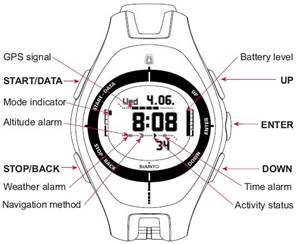
Figure 1 Layout of the X9,
display elements and buttons. The X9i does not have the white sighting marks at
the black edge of the display.
Each
DISPLAY MODE contains a related MENU of several selectable functions. These Menus
are accessible in each DISPLAY MODE with a short press on the ENTER button. E.g. if you want to record the GPS coordinates
of your journey, you navigate first (with UP or DOWN buttons) to the ACTIVITY
DISPLAY MODE, then press on ENTER. This specific ACTIVITY MENU is shown in Figure 2:

Figure 2 ACTIVITY MENU. The
reverse font shows the option that is selected if one press again on ENTER.
In this
ACTIVITY MENU the first function shows ‘ACTIVITY’. In Figure
2 above, the ■ (no record) is set. By pressing again
on ENTER, the option is shown in reverse font and can be changed into ► (record) or ▌▌ (pause) by using the UP and DOWN
buttons. Assume you select ► (record) and press on ENTER again. The track log then starts by saving
the time of the day in the header. If the GPS receiver was not yet activated,
it will start seeking the satellites. To show this, an empty squared box starts
blinking on the first line. Once a satellite FIX is established, the blinking
empty box is replaced with bars (black boxes). One bar means that the GPS
signal reception is very weak; five bars denote a maximal signal reception strength.
On the Figure 3, four bars are shown, indicating that the received
signal strength is very good.
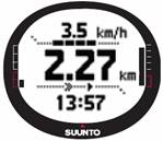
Figure 3 Activity window when GPS is on.
I have experienced that in order to obtain a valuable track log one needs at least three black boxes. If the signal reception is weaker, then the position error of the recorded track points raises, and the track log will show inaccurate positions.
Select the STOP-BACK button to navigate back from a SUBFUNCTION to a higher function and back to one of the five DISPLAY MODES.
There is
also a sixth (hidden) display mode, accessible from either DISPLAY MODE by a
long press on the enter button:
6. POSITION FUNCTION DISPLAY
MODE to MARK (record)
specific MEMory points; find the recorded HOME MEM point; or to observe your current
GPS position and signal quality ( Figure 4):
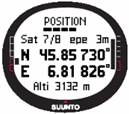
Figure 4 Subfunction POSITION of the POSITION FUNCTION DISPLAY MODE
This display shows the following data:
Ø The four bars ■ ■ ■ ■ indicate a strong GPS satellite signal reception strength;
Ø
Sat 7/8 shows that 7 satellites are fixed,
and that 8 satellites
are received. So there is one satellite not yet fixed.
Ø epe 3m displays the estimated position error derived from the fixed satellites signals;
Ø Coordinates display the latitude and longitude in any format you want. The specific format is to be set in the UNITS subfunction of the TIME DISPLAY MODE.
Ø
The last line can display two
parameters (by toggling on
the Start-Data button):
o Alti displays the GPS altitude. (The display units of this parameter can be set in the UNITS subfunction of the TIME DISPLAY MODE). GPS altitude readouts are not stable right away, therefore, even with 7 satellites FIXED and high signal strength, it takes a little while to trust this number.
o
The elapsed time to the first satellite fix.
If the GPS
receiver is paused, stopped, or when there is no fix, the coordinates of the last
GPS position are displayed. These position coordinates are updated when the device’s
position changes and another FIX is established.
Note: Even with a strong GPS signal (3 bars or
more; e.g. ■ ■ ■ ■) and much satellites in direct view
(at least 4, e.g. 5/5), it is possible that the epe is high (e.g. 25 meters). The reason can be:
1. the correlation has not been
finished yet. The epe will reduce during the next seconds and minutes;
2. when the epe remains high, then probably the satellites are not well spread (to
much aligned)
Changing a
DISPLAY MODE will change the display of the X9i, but not the tasks you have ordered
to the X9i. So you can easily navigate
to the TIME DISPLAY MODE, while navigating to a WAYPOINT and recording the
track log in the background.
Besides the
1 to 5 bars showing the current signal strength ( ■ ■ ■ …),
other symbols can appear as well on this line:
1. When the GPS receiver is activated, the line showing the signal
strength can also show a different symbol:
□
(blinking
empty box) : The activated receiver is trying to establish a GPSFIX.
2. When the GPS receiver is in sleep
mode, then the line
showing the signal strength can show two different symbols:
□
(not
blinking empty box) : The last GPSfix was not successful to propose a valid
location;
![]() :
The last GPXfix found a valid location
:
The last GPXfix found a valid location
3. When the GPS receiver is OFF, the line does not show a symbol.
This signal
strength line is also visible in the NAVIGATION DISPLAY and the ACTIVITY
DISPLAY.
3.2.2 Setting up the displayed GPS UNITS
If the
reader is novice to GPS, it is advised to read first the appendix chapter 12. If one understands the meaning of a map DATUM,
position and geographical coordinates, one can proceed with this section.
|
It is only necessary to set the DATUM and
position coordinate system in the X9i if one wants to work with the position
coordinates in the X9i: Ø
when one reads the current GPS location (in the POSITION SUBFUNCTION) and
wants to interpret this on the printed map; Ø
when one adds/edits, from the printed map, ROUTES or WAYPOINTS
directly in the X9i (to navigate on). ONLY IN THESE TWO
CASES it is necessary that the MAP DATUM and position coordinate
system in the X9i corresponds with the printed map grid and DATUM. |
Then there
will be a one-to-one relationship between the displayed coordinates on X9i and
the grid position coordinates of the printed map.
If UTM coordinates
are set on a WGS84 datum then you need to have a map with UTM grids lines over
the whole map. If not, you can not
observe where you are on the map. Since UTM grids are not commonly used
throughout the world, it is necessary to
check this in advance (and adapt the displayed GPS coordinates accordignly).
This is discussed in Section 3.2.2.2.
If one
always program the ROUTES and WAYPOINTS with external software (Suunto Trek
Manager, third party software (that eventually have X9i drivers embedded), and
one is also not going to interpret the Position subfunction (Figure 4 ), then it is not necessary to set the GPS Datum
and position coordinate system.
In fact,
the X9i is designed to navigate not by displaying the position coordinates, but
by displaying the current distance and direction to the next waypoint. So, in
most cases, the MAP DATUM and position coordinates in X9i are to be set
correctly only if one has to do an on-the-field programming of Waypoints/Routes in X9i.
The
Displayed GPS UNITS are set in the TIME DISPLAY MODE, function UNITS, SUBMENUS
DATUM, POSITION and GRID.
3.2.2.1 Available datums and position
notations in X9i
The X9i can
handle 255 different MAP DATUMS. A list is given in Chapter 9 (page 88 to 95)
of the X9i user manual, downloadable from this link http://www.suunto.fi/suunto/main/article_1column.jsp?JSESSIONID=ERCR2OBKRdAk1t9vy8R575ZfebzP1LGyw84ZGKGTe06g417bln3m!-236121259!168075286!7005!8005!347035074!168075285!7005!8005&CONTENT%3C%3Ecnt_id=10134198673939518&FOLDER%3C%3Efolder_id=9852723697223448&PRODUCT%3C%3Eprd_id=845524442492820&bmUID=1150386897249
. A few examples are given in the following list:
|
Selection number in X9i |
Datum description in X9i manual |
printed MAP datum label |
|
255 |
WGS84 World Geodetic System 1984
(most widely used) |
WGS84 |
|
071 |
EUR-A ( |
ED50 |
|
099 |
NAS-C Mean Solution (CONUS) |
NAD83 |
|
068 |
AUG |
AGD84 |
|
… |
… |
… |
Table 1 Subset of available
map DATUMS in X9i
The X9i can
also handle a variety of position coordinate systems. The following table
classifies them:
|
Format notation in X9i |
meaning |
|
Deg |
In latitude and longitude degrees
(decimal format) |
|
Dm |
In latitude and longitude degrees
(degrees, decimal minutes) |
|
Raster |
A specific local planar coordinate
system |
|
UTM |
Universal Transverse Mercator
coordinate system |
|
MGRS |
Military Grid Reference System |
Table 2 Available position formats
in X9i. The format notations with blue background (i.e. the
geographical coordinates) can be used for every available Datum. The
format notation with grey
background (Raster) does not need a Datum assignment. The format
notations with green
background (i.e. the planar coordinates) can be used for only a small
subset of the available Datums in X9i.
Deg and Dm
are geographical coordinates. Raster, UTM and MGRS are planar (x,y)
coordinates.
Raster
coordinates are different to UTM or MGRS in that way they are not defined with
a global datum (ellipsoid) but rely on a local datum. This Raster option in X9i
can be used if you specific MAP only shows a local raster (coordinate system).
Since local rasters already embed a local DATUM and projection method, it is
not necessary to assign a DATUM in X9i if you assign the GPS coordinates to a
Raster.
There are
10 local Rasters available in X9i:
|
Description of the 10 local RASTERS |
Notation
in X9i |
|
Finnish National grid KKJ 27 |
Finnish |
|
Swedish national map projection RT
90 |
Swedish |
|
British National grid |
British |
|
Swiss National grid |
Swiss |
|
Irish National grid |
Irish |
|
|
NZTM |
|
Royal Dutch grid RD |
Dutch |
|
Austria Area grid M28 |
BNM M28 |
|
Austria Area grid M31 |
BNM M31 |
|
Austria Area grid M34 |
BNM M34 |
Table 3 10 available local
rasters (Grid) in X9i
There are a
lot of existing local grids that can’t be set (E.g. the Belgian local grid
Lambert 72 based on the local datum BD72 is missing). Fortunately these printed
maps also provide other grids (in general UTM) in printed overlay. Then it is
often possible to use the other printed grid.
If the
printed grid can’t be used in the X9i (because the Grid or the Datum is not
available), then one has to add manually on then map the geographical grid by
using the geographical tick marks along the map. Such an example is given in Section 10.1.
3.2.2.2 How to set correctly the datum and position
format in X9i?
This
section is extremely important (a must know) if your maps aren’t made with a
WGS84 datum and no overlaying UTM gridlines are visible (face different real
life datums in Section 12.1). So most X9i users should read this, or they misuse
the X9i.
3.2.2.2.1 Problem statement
Most of the
GPS softwares can combine hundreds of map datums with planar and geographical
coordinates. STM also can combine 255 DATUMS with all the regular position
coordinates (planar and geographical). The X9i however does not support planar
coordinates for all the 255 DATUMS, but only for 7 DATUMS (memory
restriction?). The available DATUMS in X9i for planar coordinates (UTM or MGRS
format) are the following;
|
Selectable map DATUM
in X9i when POSITION format is UTM |
|
|
|
|
|
|
|
WGS84 |
|
NAD83 |
|
NAD27us |
|
NAD27ca |
Table 4 7 available Datums
in X9i when UTM or MGRS position coordinates are used
It
is a pity that the X9i only can use UTM grids on so few DATUMS. Some really big
Datums like European Datum 1950 (ED50) is just missing in this list. As result,
a whole continent is a virtual candidate.
Remark:
When you
set the DATUM of the X9i with the Suunto Trek Manager (STM), you will see that
there are more DATUMS available (15 instead of 7, so 8 are missing in X9i):

Figure 5 15 available Datums in X9i if one uses STM.
When you
select one of these 8 missing DATUMS in STM (E.g. NAR-B), and one updates the
X9i settings, then the function DATUM in X9i shows a blank field. I don’t know
what kind of coordinates is produced then on the X9i display. I guess this is a
firmware/software bug and this situation is to be avoided.
3.2.2.2.2 Correct assignment procedure
The
following flow chart finds the best possible match between the printed map
compilation notes and the the X9i Datum
and Position format -or Grid- units.
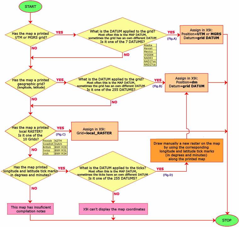
Figure 6 Flow chart assigning the Position and Datum, or the Grid, of the
X9i from a printed map
This
document shows different printed maps with their correct assignments:
(Fig.A): Figure 60 of Section 6.3.1: DATUM=WGS84,
Position=UTM
(Fig.B): obsolete.
(Fig.C): Figure 84 of Section 12.2: Grid=RD
(Fig.D): Figure 72 of Section 10.1: Datum=ED50,
Position=dm
Due to the
advent of GPS, almost all carthographic institutes tend to switch from geographical
grids to UTM grids. This is why geographical grids on printed topographical
maps are obsolete.
3.2.2.3
An
example showing the assignment procedure
Figure 7 shows a regular topographic map of a part of
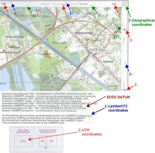
Figure 7 Printed topographic map: DATUM and Position selection of the X9i
The map
compilation notes show:
Ø
MAP
DATUM is ED50 (“1951 Unified European Geodetic System”).
Ø
There
are three different position coordinate formats applied on this ED50 Datum:
1:
Tick marks at the outside: the original position format (local projection
system) is Lambert72. Lambert72 coordinates are not available in X9i.
2:
Tick marks at the inside: geographical coordinates (longitude and
latitude angles)
3:
In overlay there is a printed red 1 kilometer UTM grid (in zone 31U).
The assignment procedure goes as follows (only
the correct path is depicted):
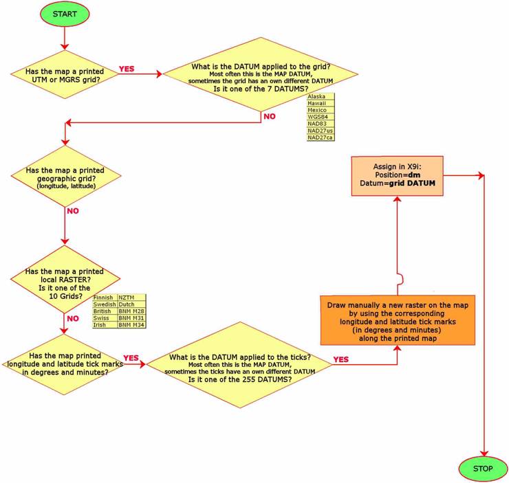
Figure 8 Assignment of the
X9i Datum and Position for a Belgian topographic map
For the assignment in X9i (TIME DISPLAY MODE,
function UNITS) it is best to set first the Position, then the Datum:
1. SUBFUNCTION Position=dm.
2. SUBFUNCTION DATUM =071. (From Table
1, the identifier 071
is found for ED50. (if the POSITION
format is not one of the geographical coordinates Deg or Dm, then identifier 071 can’t be set).
The assignment procedure informs that there is
an additional geographical grid to be drawn. This is necessary because the
printed UTM grid can’t be used to resolve the displaying coordinates in X9i,
which are restricted to latitude and longitude degrees in the map Datum ED50.
To do this correctly, the tick marks of the same value, lying at the opposite
side of the map, are to be connected. Because this specific map is cut out parallel
to the longitude and latitude angles (See Figure 9 to the right), this addition is relatively easy.
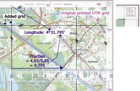
Figure 9 Adding a geographical grid to a map with ED50 datum. Finding the geographical coordinates of a point of interest (a bridge).
Note that this kind of map cut out is not
general: Most of the time the map cut out is done along the UTM grid, making
the geographical tick marks slanted on the map.
If one assigns to ‘Position’ the Dm format instead of the Deg format, then the decimal fraction between the grid lines does not need to be converted to integer seconds.
A mistake easily
made is that one assumes a WGS84 DATUM when one reads UTM coordinates on a map.
An illustration of the effect involved is given in Section 12.3.
Note again that if you do not look at the
POSITION SUBMENU in the POSITION FUNCTION DISPLAY MODE, and you are not
planning to program WAYPOINTS or ROUTES on the X9i display, then you do not need
to bother all the above settings. The X9i will record the GPS coordinates
(probably in UTM/WGS84) properly, and all the software’s that download track
logs from X9i know in which format/Datum the track log is saved.
3.2.3
Setting
up the current time
The best
method to set the time is activating the GPS, and then add the UTC time offset
for your specific location. To do this,
Ø
Navigate
to the TIME DISPLAY MODE, function TIME/DATE, SUBFUNCTION SYNC. There set the
sync ‘on’;
Ø
Being
still in the function TIME/DAT, select the SUBFUNCTION UTC. There set your UTC
time offset (and account for possible additional summer time shift).
Every time
there is a GPS FIX, the displayed time will be adjusted.
If you
don’t know your UTC time offset, you can look at the GPS synchronized time and
the difference with your current time. Then you can adjust the displayed time
by modifying the UTC time offset.
If the UTC
time offset is less than 30 minutes, you will have to set the current time by
adjusting it manually, and then set the sync ‘off’.
3.2.4
Setting
up the X9i with STM
In Section 5.1.2.1 it is explained how you can set up the X9i with the
Suunto Trek Manager.
There is
one setting you can’t do on the X9i display, although it is mentioned in the
manual: TIME DIOSPLAY MODE, function GENERAL, function INFO. This is to be done
with STM.
There are
also a few settings that can’t be set in STM, like the NAVIDATA selection (see Section
7.2) and GPSFIX selection (next Section 3.3).
3.3 GPS FIX
You will
need to do an initial GPS FIX when the satellite constellation is changed
significantly:
1.
you
haven’t used your X9I GPS for a few weeks, or
2.
If
you changed your location for more than 200 kilometers.
Then the X9i will need to gather additional
data after a GPS FIX, to be able to estimate correctly your position. To do
this, place the X9i on a flat surface with the face pointing towards the sky
and leave it in this position for at
least 15 minutes. The progress of this FIX can be observed in the POSITION
submenu. After this, you are allowed to move your X9i.
To do an initial GPX FIX, do the following:
1.
Go
to the ACTIVITY DISPLAY MODE, function GPSFIX. Set this to 1 sec. Other options
are 1 min and manual, but for this purpose the X9i needs to do a continuous
update of the GPS receiver, and hence 1 sec fix is mandatory.
2.
Then
long press on enter to go to the POSITION FUNCTION DISPLAY MODE, and go to the
GPS MENU. Set this to ‘on’.
3.
(Eventually
navigate in the same POSITION FUNCTION DISPLAY MODE to the function POSITION;
this will let you observe once in a while the signal reception strength, the
number of satellites received and fixed, and the position error.)
4.
Most
important is to place the X9i somewhere fixed with its display directed
vertically. Do not hold the X9i on your
wrist as it increases significantly the elapsed time to a first fix of the
received satellites, as well as the other data collection.
The best position to place your X9i is one that
allows a FIX for at least 8 satellites. If this seems not possible, then look
for another place where buildings, trees, etc do not hinder the direct view of
the satellites from the X9i.
After having done an initial GPS FIX,
subsequent FIXes do not have to wait an additional 15 minutes for data
collection.
From a practical point of view I experienced
the best results by doing as follows:
|
1.
Always do a GPS FIX off-wrist, from a fixed location with clear view
on the sky. Then the GPXFIX only takes around a minute, and the quality of
the position estimations will be at its best. 2.
Be sure the GPX FIX is established with good signal reception strength
(at least three signal bars, preferably four), and that at least 6 satellites
were fixed. The duration of this fix should be sufficient to have an epe of 1
meter. |
The high
signal strength in conjunction with the clear sky view, will lead to a fix of
all the current observable satellites.
When for some reason some satellites aren’t received temporarily
thereafter, the X9i will catch up the fix within a few seconds when the hidden satellites
are again visual.
4
Recording
Tracks, ALTitude, MEMory points and other data
The X9i can
record up to 24 tracks embedding positional and altitude data over time (see Table 7 in Section 9.5).
The X9i
records data when ACTIVITY DISPLAY MODE, function ACTIVITY is set to record ►.
During such
a recording state, there are a lot of things that the X9i records:
1. When the GPS receiver is active, the
X9i can record a track log. This is a history file of where you were (position
and altitude) at what time. In the next
Section 4.1 it is explained how this sampling effectively takes
place.
2. Independent of the activation of the
GPS receiver, the X9i records as well the altitude with a different and fixed
sampling rate (see the 4th column of Table 5) in the next section. Consequently, when the GPS
receiver is active, the X9i records twice the altitude: once in the track log,
and once in a separate altitude array. When the GPS receiver is off or in sleep
state, the altitude recordings still take place in the separate altitude array.
3. Memory points are stored individual
positions of relevant locations. Memory points differ from track points in that
way they do not have a time stamp. The fundamental display to manage a MEMory
point record is the POSTION FUNCTION DISPLAY MODE. Memory point recording is
discussed in Section 4.2
4. Additional data is recorded as well,
like the time stamp of the start of a record (►), every time the activity is paused
(▌▌) or continued (▌▌), or when the activity is stopped (■).
4.1 Recording Tracks and ALTitude
Once your X9i has had an initial GPX FIX, you
can start to record your first track (ACTIVITY DISPLAY MODE, function ACTIVITY,
set to record ►). The
position is recorded by correlating the GPS signals in the GPS receiver, the
altitude is estimated indirectly by a sensitive and calibrated pressure sensor.
The altitude is stored in the Track log as well as in the separate altitude
array.
The
different recording cadence of the track log and the altitude array is given
in Table 5, and can be observed in the Suunto Data File export
file from STM. This file shows a section [POINTS] with on each row the “TP”
track points at the date and time stamp of each record. There is as well a
section [CUSTOM1] with on each row the elapsed time from start of the record
(in seconds) and the current altitude.
One can observe that each “TP” as well contains an altitude field. Since
the altitude recording does not depend on track points recording rules, the
recorded altitude array has a higher recording frequency than the recorded
track points. As it is shown in chapter 5, it is the recorded altitude array that is used to
depict the altitude graph in STM.
4.1.1 Accurate position recording
4.1.1.1 Start a track log AFTER the ACTIVITY is set to ►
The X9i can start to activate the GPS without
using the POSITION FUNCTION DISPLAY: By starting a track log from the ACTIVITY
DISPLAY, function ACTIVITY (set to record ►), the X9i records the start time,
and if the GPSFIX is not set to ‘manual’ (see Table 5), the GPS receiver is activated automatically. If you
then start your journey, you start to use the X9i in bad initial conditions.
Therefore I do not recommend this kind of ‘record initiated GPS start’. It is
always better to establish a GPS FIX with your X9i on a fixed surface and
having the maximum number of satellites fixed (clear sky).
4.1.1.2
Continue
a track log NOT by setting the GPS ‘on’
If you have paused (▌▌) the GPS during the same journey,
you may NOT decide to start the reactivation of the GPS receiver the
recommended way (i.e. by setting GPS from ‘off’ to ‘on’). This would stop the
track log and start a new one. So, when
you need to continue your track log, you will have to switch the track log pause
(▌▌) to record (►), which will continue the record of
the track points in the same track log.
4.1.1.3
GPSFIX,
recording intervals, memory capacity, battery lifetime
The X9i can store up to 25 different track logs,
and up to 8000 track points.
The most important setting for a record is the
GPS FIX rate (ACTIVITY DISPLAY MODE, function GPSFIX). This can be set to 1 sec,
1 minute and manual. In Table 5 shows what the manual says about these different GPS
FIXes:
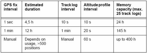
Table 5 Influence of GPSFIX on the battery consumption, track log and altitude recording, and X9i memory
I found that, on the average, the battery consumption is in agreement with the first row of this Table (1sec GPSFIX): I was able to use a GPSFIX for 4 to 5 hours, until the GPS receiver switched itself into manual mode.
The 1 min and Manual GPSFIX can easily show much smaller durations. This happens when the signal reception occurs in weak conditions: Normally, when there is a clear view to the sky, a GPSFIX and position estimation build up, takes around 10 sec to 45 sec. When there is no clear view to the sky, this operation takes much more time. As result, for a 1 min GPSFIX, the estimated duration of 12 hours will not be reached. 7 to 8 hours is a more realistic number in these cases.
In section 4.1.2.2 it is shown that the best GPSFIX setting for track log recording in very demanding situations (deep canyons, heavy rain in dense woods) is manual.
The lack of an on the field charging facility is a weak point of the X9i design. Fortunately it is relatively easy to fabric by your own an on the field charging unit: see Section 9.
The track log interval depicted in Table 5 shows the simplified rules of the recording process:
E.g. for a GPSFIX=1sec: record every 10 sec. But only if that is necessary (if there is no move, then don’t record a next sample) and possible (wait to record a next sample until the GPSFIX quality is sufficient).
The following recording rules can be detected when a GPSFIX of 1sec is set:
1. When the GPS signals do not conclude that a change of the position occurs, no track point will be recorded after 10 sec;
2. When the GPS signals still do not indicate a change of the position after a minute of that last track point record, a new track point record takes place;
3. When the X9i is does not receive any GPS signal (i.e. no fix, blinking indicator) for a certain period, and then no track point is recorded.
4. When the X9i has no fix during 15 minutes consecutively, then the GPSFIX will be changed automatically into MANUAL..
Rule 1 to 3 saves memory space; rule 4 saves battery power.
When a 1 minute GPSFIX is set, the X9i activates the GPS after one minute of the last successfully recorded track point. As result, at that event of awaking the GPS receiver, it takes a little time to establish a fix (blinking indicator is displayed). Then, after a first satellite FIX, there is a build-up time to fix even more satellites to reduce the position error epe. The next track point will be recorded until the received GPS signals are sufficient strong, and produce sufficient accurate position estimation (=high fix quality). This processing time results in a track log that has in general no track points recorded at the cadence of one minute; except for records for a good signal quality.
When a manual GPSFIX is set, the power demanding process of GPS reception can be invoked at user interaction (long press on STOP/BACK in NAVIGATION and ACTIVITY DISPLAY MODE.
As result, the memory capacity is in reality bigger than the numbers depicted in the Table. E.g. the maximum of 8000 storable track points can cover at least 8000*10 seconds=22h13 min. By accounting for the recording rules, the 24 hours recording time is a minimal expectation.
The GPSFIX can be modified on the fly. Some examples where this modification is valuable:
1. when the battery remaining power seems to be insufficient, you can switch to GPSFIX from 1sec to 1min or even manual mode in the same track log record.
2. when the pathway changes from a clear view to the sky to a dense forest or a deep valley or canyon, then it is better to switch the GPSFIX to 1 minute or even manual.
3. when the pathway is a straight line without turns, it is sufficient to do a GPSFIX at both sides of the straight line.
.
4.1.2 Accurate altitude recording
It is well
known that the altitude readout from instant GPS measurement is not applicable
for the instant recording of the true altitude (http://gpsinformation.net/main/altitude.htm
). Even if the instant GPS altitude could be estimated in a more stable and
accurate way, the altitude displayed would be off the altitude displayed on a
topographical map. This is because different zero references are used (see
Chapter 12).
As result,
the X9i is designed to display and record the barometric altitude instead of
the GPS altitude. It works like this:
1. Assume the X9I is set to ALTI (USE ALTI). Then a change of air pressure is
treated as if it is due to a change of altitude. This altitude is displayed on
the middle line of the ALTI/BARO DISPLAY.
Þ When a track log record is started, The ALTItude displayed on the
ALTI/BARO DISPLAY is also displayed at the lower line of the ACTIVITY DISPLAY
(selectable with STOP/BACK). This value is recorded in the track log as well as
in the altitude array.
2. Assume the X9i is set to BARO. Then the ALTitude is kept fixed by setting an
ALTITUDE REFERENCE. The changes of the barometric pressure are interpreted as a
change of air pressure at the REFERENCE. The lower line of the ALTI/BARI
DISPLAY can display this pressure (with STOP/BACK button). The upper line
displays the equivalent pressure at imaginary sea level, useful to forecast
weather.
Þ When a track log record is started, the ALTI/BARO DISPLAY will be kept
unchanged (pressures are visualized), but the ALTitude REFERENCE is released, and the current
pressure becomes fixed. From then on, every change of air pressure is treated
as if it is due to altitude changes. These changes of altitude are displayed at
the lower line of the ACTIVITY DISPLAY (selectable with (STOP/BACK). This value
is recorded in the track log as well as in the altitude array.
When the recording of the track log is stopped,
the current ALTItude is assigned to the ALTITUDE REFERENCE and the current air
pressure will be released. From then on, the changes of air pressure will have
no influence any more on the ALTItude.
Consequently, if you set USE BARO and set the
ALTITUDE REFERENCE to a certain height, a track log record will release this
reference and adapts this value if you change height. When the record is
stopped, the new ALTITUDE REFERENCE is then different to the previous REFERENCE.
That way, the X9i keeps track of the changes of the altitude during a record.
4.1.2.1
Influences
on altitude measurement: barometric drift and ISA
The manual
of the X9i estimates that the GPS altitude readouts have an accuracy of 2 times
the accuracy of the other position coordinates (after a quality fix). Consequently, the X9i does not record the GPS
altitude (observable at the lower line of the POSITION FUNCTION DISPLAY MODE,
function POSITION) but it records the indirectly measured altitude obtained
from the effect on barometric pressure.
This offers a very accurate measurement of changes in altitude for relatively
stable weather conditions. Normal
weather conditions also involve a barometric drift that can be the equivalent
of 10 to 20 meters in one day. When the weather is unstable, then the
barometric drift can cause an equivalent over 10 meters in a few hours.
The
ALTI/BARO DISPLAY MODE, function ALARM offers two alarms:
Ø
SUBFUNCTION
ALTITUDE AL offers an alarming signal when the altitude exceeds a threshold
altitude;
Ø
SUBFUNCTION
BARO AL offers an alarming signal if the X9i measures a barometric drift that
equals the generally accepted threshold for unstable weather (10 mbar over 3
hours)
Of course,
the BARO AL is only valuable is one stays around the same altitude. In this
case, I found it a very useful instrument to forecast rapidly changing weather
in the next 24 hours.
There are a few precautions if one tries to
record accurately the changes of altitude by measuring air pressure:
1.
It
is not a good idea to set the altitude at the start always to 0 meters. This is
because a change in pressure of 10mbar is related to a change in altitude of
around 87 meters at sea level, and around 118 meters at 3000 meters altitude.
2.
Second,
the temperature is not constant for each altitude. The International Standard
Atmosphere ISA (e.g. http://www.aeromech.usyd.edu.au/aero/atmos/atmos.html)
shows that the air temperature gradient in the troposphere is around 6,6Kelvin
per 1000 meters. The sea level conditions show a temperature of 15°C at an
absolute pressure of 1013 mbar. (http://www.aeromech.usyd.edu.au/aero/atmos/atmtab.html
). The influence on altitude measurement on pressure sensors is calculated in http://www.biber.fsnet.co.uk/altim.html.
I think that
the pressure sensor in the X9i is calibrated to cover these ‘normalized’
changes of air pressure and temperature (the old SUUNTO advisor already had the
same ‘calibrated pressure sensor’).
4.1.2.2 Guidelines to obtain very accurate estimations
of the altitude
In order to
estimate accurately the altitude, it is necessary to set first correctly the
Altitude RFFERENCE at the start of a trip (ALTI/BARO DISPLAY MODE, function REFERENCE,
SUBFUNCTION ALTITUDE (SUBFUNCTION sea level is missing). Hence, to set
correctly the true altitude, the best method is to read from a topographical
map the current altitude at the start.
(A second best method is to read the GPS
altitude at the start (lower line of the POSTION FUNCTION DISPLAY MODE,
function POSITION) by taking extreme care to GPSFIX as much as possible satellites.
The longer the GPSFIX lasts, the more accurate the GPS altitude will be (this
takes time). Supplementary, one should look after the specific difference of
the true sea level used for topographical altitude reference (geoids altitude)
and the GPS altitude reference (altitude above the GRS80 ellipsoid of the WGS84
DATUM), see Chapter 12).)
When one
expects temperatures that are off the normalized values of the ISA, then the
altitude readouts will differ slightly with the true altitudes. In the Yahoo WriststopTrainers forum http://health.groups.yahoo.com/group/WriststopTrainers/ this has been discussed by member Bruce. Based on his communication and the
approximations made in the Suunto Advisor manual, I derived an equation that estimates
the error on the altitude when the air temperatures do not correspond with the
normalized ones:
![]()
Equation 1 CORrection factor
accounting for not normalized temperatures at different events of a trip
With:
§
A2_ISA is a better estimate of the altitude at event
2, accounting for the deviations on ISA between the two events 1 and 2.
§
T1 the correct
air temperature (in °C) at event 1 of the trip;
§
T2 the correct
air temperature (in °C) at event 2 of the trip;
§
A2 the measured/displayed
absolute altitude (in
m) at
event 2 of the trip;
§
A1 the correct
absolute altitude (in m) at event 1 of the trip. This must be the altitude on
which the X9i is calibrated, hence the displayed altitude at event 1 equals the
correct absolute altitude at that event 1.
§
COR the correction (in m) on A2 to find A2_ISA
T1 and T2 can be
measured with the X9i by observing the temperature on the display (ALTI BARO
DISPLAY MODE, lower line –eventually after switching this line content with
STOP/BACK- when the X9i is at least 40 minutes off the wrist and in the shadow.
Read MSG2626
for the equivalent equation in °F and feet units.
A graphical
representation of this equation is given in Figure 10:
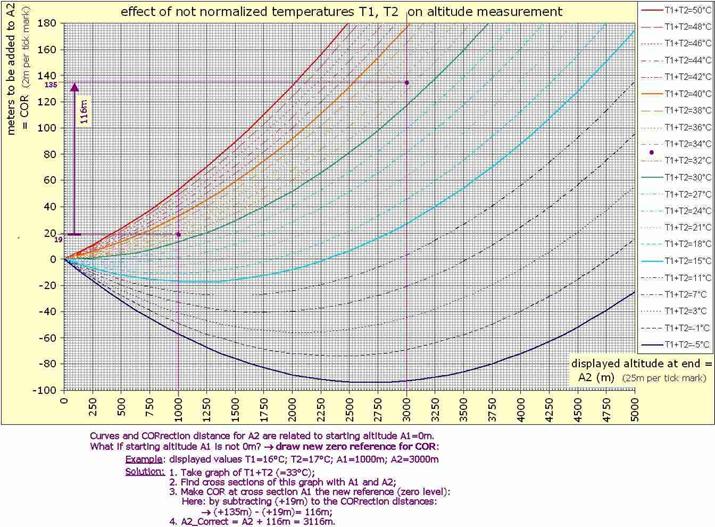
Figure 10 Pressure calibration chart, useful to derive the correct altitude at the end point based on measured barometric altitudes and true temperatures at the start and end point. This chart (and as well the (°F, feet) version) can be downloaded separately from the location http://health.groups.yahoo.com/group/WriststopTrainers/files/WM%20Stuff/ .
A possible alternative to correct the
displayed altitude at the end point is to observe the stabilized and accurate
GPS altitudes at start and stop positions. In that case, to minimize the altitude
error, I feel that the signal strength reception and the number of fixed satellites
has to be maximal (at least four bars, at least 7 satellites fixed, epe maximal
1 m). Then, by making the difference between the two stabilized GPS altitudes,
the altitude at the end position can be found by adding that difference to the
correct altitude at the start position.
4.1.2.3 Altitude measurements at the same spot
The
barometric drift will result in changing altitudes at the same location. But is
is not ‘only’ the barometric drift that affects this changing altutude; ISA
affects this as well. It is possible to find a rule of thumb that finds the
proportion of this ISA on altitude measurements if one measures at the same
altitude:
For -5°C < T1+T2 < 50°C, the effect of changes of air
temperature on changes of altitude readouts is maximal 6%;
For 10°C < T1+T2 < 40°C, the effect
is even much smaller: 3% at most for quite a lot of altitudes
Reason: look
at the highest slopes of the curves in the relevant altitude regions:
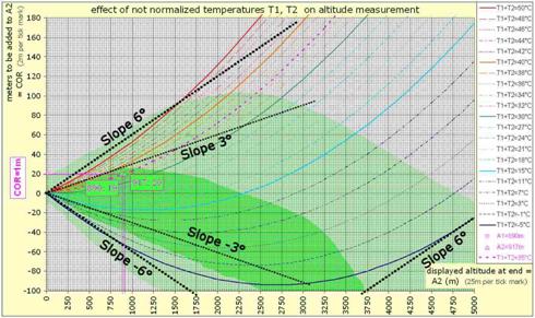
Figure 11 The change of
measured altitude at a spot (where X9i is calibrated) is due to the barometric
drift and deviations from ISA (shown in this figure). Light
green zone: deviations form ISA show a correction of at most 6% * displayed altitude difference. Dark
green zone: deviations form ISA show a correction of at most 3% * displayed altitude difference.
One can
conclude that most often the changes of the measured/displayed altitude at the
same spot are for at least 94% (97%) due
to the barometric drift. Because the displayed altitude differences at the same
spot are relatively small in normal weather conditions, we can neglect effects
due to ISA.
Example: Assume one stays at 890m altitude
and calibrates the pressure sensor to 890m at an air temperture of 12°C. 7
hours later the X9i altitude shows at the same spot 917m at an air temperature of
23°C:
§
The rule of thumb says T1+T2=12°C+23°C=35°C, hence only
maximum 3% of the change of altitude is due to deviations from ISA:
(917m-890m) = 27meter
27meter * 2% = 1 meter (negligible)
Correcting the measured altutide after 7 hours for deviations to ISA (negligible):
917m+1m = 918meter
§
The correct formula (Equation 1) shows the proof:
![]()
Þ
The
change of the altitude due to the barometric drift (negligible difference):
918m-890m = 28 meter
Note that a
‘temperature compensated’ pressure sensor indicates that the temperature of the
pressure sensor itself is compensated. This means that these sensors compensate
for body heat (when wearing it on the wrist) or sun radiation (when wearing it
in direct sun light), but not for changes of the ambient air temperature.
4.1.2.4
A
few practical examples
Parts of
the measurements were done by car or by rack railway. This has been done
deliberately to measure big altitude differences: In general, the bigger these
differences, the bigger the temperature compensations are.
4.1.2.4.1 Example 1: Pic de Moufons
1. Recorded data (in correct order in time):
a. START altitude
(= altitude set in X9i, read from topographic map) = 890m
Temp = 12°C
b. Moufons ALT = 2861m
i.
ALT
X9i = 2785m
ii.
Temp
= 8°C
c. Back to START position (890m), after 7 hours
i.
ALT
X9i = 917m
ii.
Temp
= 23°C
2. Analysis:
Þ
Barometric
drift
Þ Account for the deviations from ISA
between event a. and c.: see Section 4.1.2.3
Þ Barometric drift over 7 hours:
918m-890m = 28m
Þ Barometric drift half way (at the
top) (= 28m/2) = 14 meters
Þ ALT2 excluding the barometric drift
= 2785m-14m=2771m
Þ
Account
for the deviations from ISA between event a.
and b. (T1+T2=12°C+8°C=20°C;
ALT1=890m; ALT2=2771m):
Figure 12 CORrection on the measured altitude A2 due to the deviation of temperatures from the ISA temperatures. Example 1.
If there was no topographic map available at the summit A2 (there was no barometric drift (very stable and steady weather), the best guess of the altitude at the summit is:
A2_best_estimate = A2_measured_with X9i_without_barometric drift + COR
= 2771m + +52m
=2823m.
Since the correct altitude A2 is known form the topographical map (2861m), one notices an improvement of the accuracy from 96,9% to 98,7%.
4.1.2.4.2 Example 2: Puigmal
1. Recorded data (in correct order in time):
a. START altitude
(= altitude set in X9i and t6, read from topographic map) = 710m
i.
ALT
GPS = 735m (signal strength 4 bars, and after waiting 7 minutes to let
stabilize the ALT in the POSITION display, epe=1m)
ii.
Temp
= 11°C
b. Nuria ALT = 1972m
i.
ALT
GPS = 1964m (signal strength 4 bars, and
after waiting 7 minutes to let stabilize the ALT in the POSITION display,
epe=1m)
ii.
ALT
t6 1935m
iii.
ALT
X9i 1931m
c.
i.
ALT
t6 = 2550m
ii.
ALT
X9i = 2550m
d. Puigmal ALT = 2911m
i.
ALT
GPS = 2839m (signal strength 5 bars, and after waiting 3 minutes to let
stabilize the ALT in the POSITION display, epe=1m)
ii.
ALT
t6 = 2837m
iii.
ALT
X9I = 2839m
iv.
Temp
= 13°C
e. Back to START position (710m), after 8 hours
i.
ALT
t6 = 744m
ii.
ALT
X9i = 747m
iii.
Temp
= 27°C
2. A first conclusion is that the t6 and X9i behave
identically w.r.t. altitude measurements:
During the whole journey they both showed the same altitudes within (at
most) a few meters difference.
I noticed that the t6 adapts much faster to
ambient temperature as the X9i. X9i
shows a correct ambient temperature after at least 40 minutes, t6 already after
20 to 30 minutes. This is probably due to a different weight of both tools.
3. Further analysis from start to highest peak:
Þ
Barometric
drift:
§
Rule of thumb : T1+T2=11°C+27°C=38°C, hence only
3% of the change of altitude is due to deviations from ISA: (747m-710m) *3% = 27m * 3% = 1m (negligible)
§
Correcting
the measured altutide after 8 hours for
deviations to ISA (in fact negligible): 747m+1m = 748meter
Þ Barometric drift over 8 hours:
748m-710m = 38meters
Þ Barometric drift over 4 hours (at
the top) = 38m/2 = 19 meters
Þ ALT2 excluding the barometric drift
= 2839m-19m=2820m
Þ
Input
for the chart: T1+T2=11°C+13°C=24°C; ALT1=710m; ALT2=2820m
Figure 13 CORrection on the measured altitude A2 due to the deviation of temperatures from the ISA temperatures. Example 2.
If there was no topographic map available at the summit A2 and if there was no barometric drift (very stable and steady weather), the best guess of the altitude at the summit is:
A2_best_estimate = A2_measured_with X9i_without_barometric drift + COR
= 2821m + +72m
=2893m.
Since the correct altitude A2 is known form the topographical map (2911m), one notices an improvement of the accuracy from 96,9% to 99,4%.
If one uses the GPS ALT differences to
compensate for the deviation towards the ISA temperatures, then:
A2_GPS – A1_GPS =
2839m - 735m
=2104m
Then the best estimate with GPS can be found
as:
A2_best_estimate_with_GPS=
A1_measured_with_X9i + 2104m
= 710m + 2104m
=2814m
For this experiment, this result still is not
as good as the one obtained by looking at the barometrically obtained altitude.
4.1.2.4.3 A last example
1. Recorded data (in correct order in time):
a. START altitude
(= altitude set in X9i, read from topographic map) = 1567m
Temp = 24°C
b. Downtown ALT = 710m
i.
ALT
X9i = 765m
ii.
Temp
= 32°C
2. Analysis:
Þ
no
possibility to measure barometric drift since it was a one way drive with car.
Þ Input for the chart: T1+T2=24°C+32°C=56°C;
ALT1=1567m; ALT2=765m
Figure 14 CORrection on the measured altitude A2 due to the deviation of temperatures from the ISA temperatures. Example 3.
If there was no topographic map available downtown at A2 then a best guess of the altitude downtown is:
A2_best_estimate = A2_measured_with X9i + COR
= 765m + -66m
=699m.
Since the correct altitude A2 is known form the topographical map (710m), one notices an improvement of the accuracy from 107,7% to 98,5%.
4.1.2.5
Conclusions
on ISA corrections
Þ
By accounting for deviations
from ISA at different altitudes, the inaccuracy of the altitude readouts
can be reduced from 3,5% to 1,5% . To manage these improvements, one
needs to know the ambient air temperature at the start position where the X9i
ALTITUDE REFERENCE is set, and at the position where the corrections are to be
known. This temperature measurement takes time. During the hike, one can make judgments
based on the start temperature.
Þ
If
one is navigating with a topographic map, then the above manipulations are only
useful of one really is unaware of the current position on the topographical
map.
4.2 Recording MEMORY points
Besides the
function to set the GPS on/off, and to display the current position, the
POSITION FUNCTION DISPLAY MODE as well has two options to record MEMORY POINTS:
1.
The
SUBFUNCTION MARK Memp will display a variety of MEMORY point names that can be
assigned in STM software to a specific location for later use in the X9i.
2.
The
In order to
record a memory point, a track log file has to record your current position. If
you don’t have a track log open, then you will first start to record a track
log. Then, if one has selected a specific MEMory point (name) to be stored, the
X9i will wait to record the current position until a high quality fix is
established (signal strength maximal, sufficient satellites fixed, epe 1m).
If you don’t want to wait for this, and accept some distance error, you
can do the record instantly by pressing on ‘enter’.
Sometimes I
noticed that the automatic recording of a MEMPOINT takes to long, even with a
high quality GPSFIX.
4.3 Instant display of the recorded data
The
ACTIVITY DISPLAY MODE shows the current speed, distance from start (via all
recorded track points), and a third number that can be set with the STOP/BACK
button: time from start (tfs),
barometric altitude, current time.
The instant
position coordinates are displayed in POSITION FUNCTION DISPLAY MODE, function POSITION;
already discussed in Section 3.2.1.
There are
also other activity displays that show information about the current log. These can be accessed with ‘START/DATA’
button in the ACTIVITY DISPLAY MODE. The information is displayed on four pages
and concerns the current activity or the last recorded one. The pages change
automatically every 3 seconds after which the device returns to the Activity
mode’s main display. The ‘UP’ and ‘DOWN’ buttons can be used to display faster
these displays. To exit the display earlier, press START/DATA again.
You can
view the following information:
1. max: Maximum speed
2. avg: Average speed
3. asc: Total ascent
4. dsc: Total descent
5. high: Highest altitude
6. low: Lowest altitude
7. runs: Total number of runs: A run is a vertical
movement of ascent or descent equaling 150ft/50m or more.
When a
track log is stopped or paused, the GPS receiver will be deactivated as well.
There are
several ways to display X9i recorded logs. Therefore you need to decide on
which kind of map you want to display the tracklog:
1. To display the tracklogs on Google
Earth digital maps, there is the Suunto Track Exporter software and other
freeware tools like GPSVisualiser.
2. To display the tracks on other
digitized maps, you need to know if the accompanying software embeds X9i
drivers to transcode X9i tracklogs:
a.
If
not, there are freeware tools like GPSBabel to solve the transcoding from
Suunto Track Manager to the input format of the accompanying software.
b.
If
available, then the software reads the data from the X9i (snake cable) and
makes the transcoding at once. Suunto Track Manager is the basic software for
this purpose, but there are other cheap and extreme efficient softwares
available.
I first
discuss the X9i tracklog displaying in softwares with X9i drivers (CompeGPS and STM (Suunto Track Manager). Then I discuss the X9i tracklog displaying a
mapping software that thas no X9i drivers. At last I discuss the X9i tracklog
displaying in GOOGLE EARTH with STE
(Suunto Track Exporter and GPSVisualizer).
5.1 Digital mapping software with X9i
drivers
There are
several digital mapping softwares that have X9i drivers. A list is given on the
SUUNTO X9i site http://www.suuntocampaigns.com/mapsite/en/ .
One of the
best digital mapping softwares that have X9i drivers and that can be used
worldwide is CompeGPS. In that regard,
I feel CompeGPS is better than SUUNTO Trek Manager (STM), partially because STM
needs a scanner alongside your PC to import a digitized version of maps in the
software (JPG, GIF or BMP format is supported). Or you will have to look for
already scanned maps that cover your tracks.
5.1.1 Displaying Tracks in CompeGPS

5.1.1.1 Setting up CompeGPS LAND
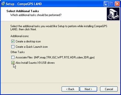
Figure 15 Installation of CompeGPS: select the installation of the X9 USB drivers.
Before pressing on Next> , be sure the X9i USB snake cable is NOT attached to an USB port of your computer.
After the installation is successful, you
can plug In the USB snake cable. After
launching
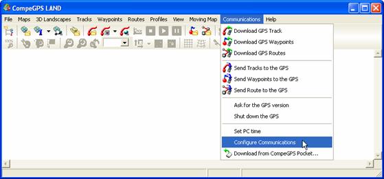
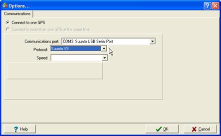
Figure 16
5.1.1.2 Reading Tracks / Routes / Waypoints
Once the configuration is done, the X9i can be attached to the USB port, and CompeGPS is ready to read/write from/to the X9i.
The example of reading a track is shown in Figure 17:
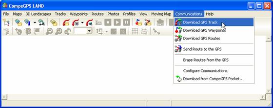
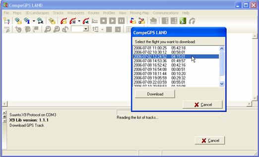
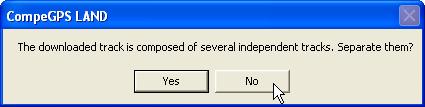
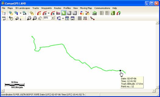
Figure 17 (TOP) after
attaching the snake cable to the PC and X9i, the option ‘Download GPS Track’ is
selected. (MIDDLE) After ‘Reading the
list of Tracks’, one can select the track to be downloaded in a separate pup-up
window. When the track log has been PAUSED, CompeGPS let you choose to keep the
parts together or split them as separate track logs. (BOTTOM) The resulting
Track is displayed in
The reading of Routes and Waypoints is quite similar, except from the fact that these are all downloaded at once and stored in their corresponding Route and Waypoints list in CompeGPS (They do not have to be selected during the import).
Opened Tracks, Routes or Waypoints can be renamed and saved in the ‘List’ option in the respective Track/Route/Waypoints pull-down menu.
Remark that listed data are not automatically saved, so save them immediately after the download.)
Once a Track is downloaded, there is a whole plethora of options and selection on this track possible. These options can be found in the pull-down menu ‘Tracks’ , or just by right clicking on the track itself (context sensitive menu). In Figure 18, altitude is selected to colorize the track:
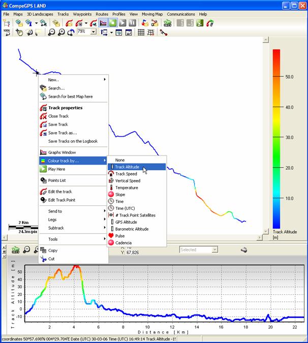
Figure 18 Context menu of a Track: Colorize Track by barometric Altitude. Graph window is displayed as well at the bottom. By selecting ‘Track properties’, various other track properties can be observed and edited.
5.1.1.3 Mapping in CompeGPS: OPTION 1: Internet servers.
One of the most interesting things of
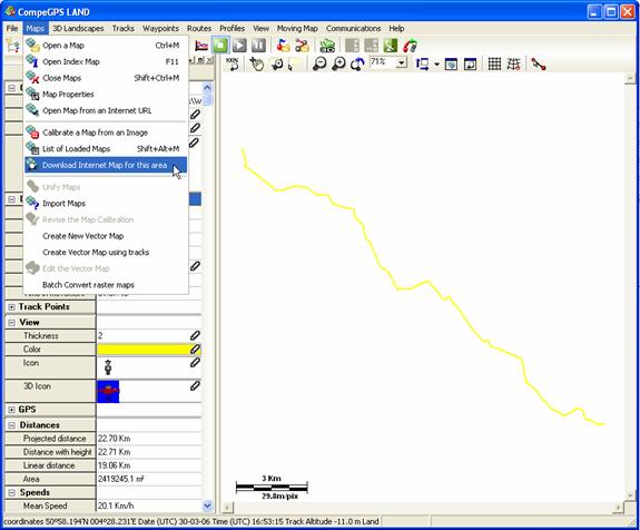
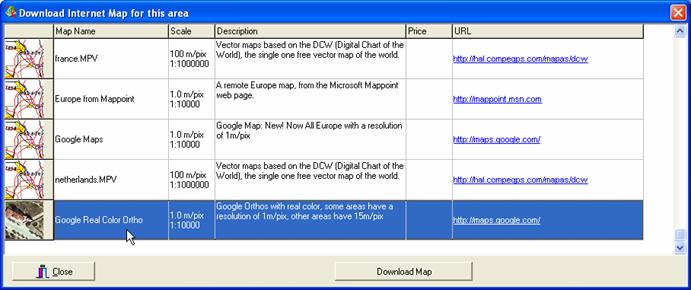
Figure 19 Downloading Internet Maps. You need to be online for this facility. CompeGPS reports back with a whole set of digital internet maps form which you can choose one of them.
In this example a Google Real Color Ortho map is selected. The result is shown in Figure 20
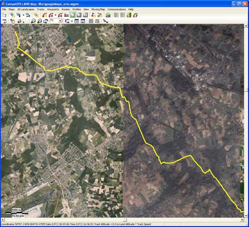
Figure 20 Imported satellite orthographic map from Google
It is also possible to download 3D maps form the internet. Therefore use the pull-down menu ‘3D Landscapes’, then ‘Download 3D Landscape for this area’, as is shown in Figure 21:
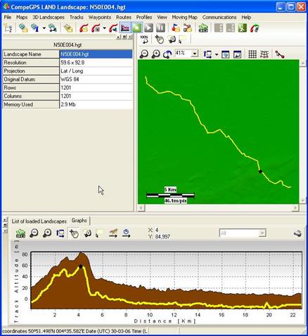
Figure 21 Shuttle Radar Topography
By selecting the Tools option in the
context menu, the measured altitude in X9i can be replaced with the downloaded
altitude data of the map. See Figure
22.
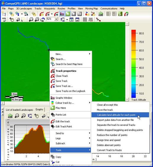
Figure 22 Replacing Altitude data
It is possible to combine all the active maps (elevation data, downloaded orthographic maps, scanned topographic maps) on the display. It is also possible to create a 3D view of such an assembly. Therefore elect the pull-down menu ‘View” and then ‘3D viewer’. This will display a 3D viewer that you can set up at your convenience. Figure 23 shows one of the results of a track on a map with elevation profile:
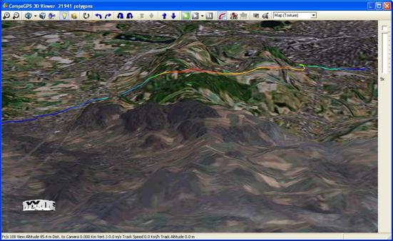
Figure 23 Track on a map with elevation data. Visualization in the 3D viewer.
Most of these maps can not be saved on you hard disk. So every time you need such a map, you will to have an internet connection.
5.1.1.4 Mapping in CompeGPS: OPTION 2: Digital maps.
Sometimes you don’t have an internet connection, or the quality of the internet map is not satisfactory. Then CompeGPS can use true digital maps in a lot of formats. These maps are loaded, either directly or using the pull-down menu ‘Maps’, then select ‘Import Maps’. See Figure 24.
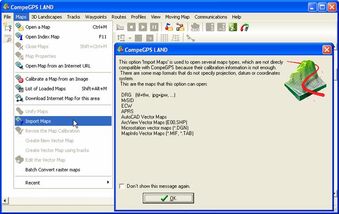
Figure 24 Importing Digital Maps
Once available, they can be used in a similar way as the maps downloaded from the internet. Except that they are always available.
5.1.1.5 Mapping in CompeGPS: OPTION 3: Scanned maps
When the two methods above are not an option, you
will need to digitize yourself paper maps. If the relevant part of the paper map is big, you
should scan it separately into parts, and then collate them digitally using a
paint/photo program. I use Paint Shop Pro for that purpose.
Warning: Both the image scanning process and
the collating is to be done with extreme care. At the end it is the aim to
obtain a perfectly aligned map without scaling and skewing differences of the
scanned parts in the map.
Note:
CompeGPS can display multiple maps at the same time as well. So if you don’t
have software at hand that can collate and rotate the individual scans, you can
ask CompeGPS to display these separate scans at the same time. However, this
asks for a little more chart calibration.
Once the
paper map is available as a scanned image (JPG or various other formats), select
the pull-down menu ‘Maps’, then ‘Calibrate
a map from an image’. Select the scanned
image to be calibrated (Figure 25):
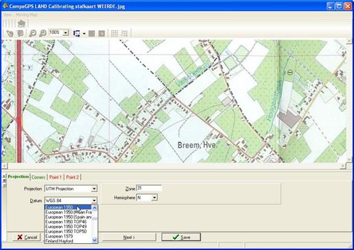
Figure 25 Starting window of
the calibration application in COMPEGPS
The scanned
map is a topographic map with compilation notes as described in Figure 7. UTM grid (on which will be calibrated) and ED50
datum are set in the first TAB ‘Projection’.
The TAB ‘Corners’ can be used to select only a
part of the map to be displayed in CompeGPS.
Then there
are two TABS (Point 1 and Point 2) in red, denoting that they are to be
assigned. The Bitmap Coordinates of a calibration are assigned by selecting a
specific point on the scanned UTM grid.
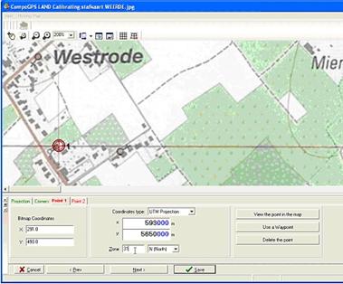
Figure 26 First calibration point in COMPEGPS
Then the
corresponding UTM coordinates are entered; and one can proceed to navigate to
the TAB ‘Point 2’ to assign another point. Calibration points should be widely spaced.
As soon a
two map points are calibrated, it is possible to calibrate more map points to
account for scanning errors and map assembly.
When ‘Create an additional Point’ is selected, the grid coordinates are
suggested based on the already calibrated map points. That way one can evaluate
immediately if it is necessary to add other calibration points.
I recommend
having at least 6 calibration points, because CompeGPS really manages to solve
scanning error issues.
Read also
the Help files to find out how you can calibrate a map in even more different
ways (e.g. by using pre-recorded position data)
CompeGPS allow calibrating maps with different datums and position coordinate systems. Once the calibration of a map is done, the calibration data is saved in an IMP file next to the image file in the folder ‘maps’.
Figure 27 shows an X9i track with the calibrated map as primary
map, and GoogleOrthoMap as secondary map.
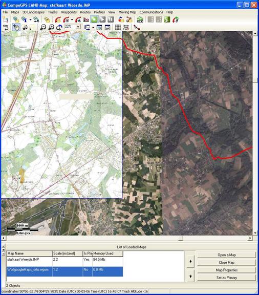
Figure 27 Mixed map
visualisation. It is even possible to modify the transparency of the primary
map.
5.1.1.6 Putting things together in 3D
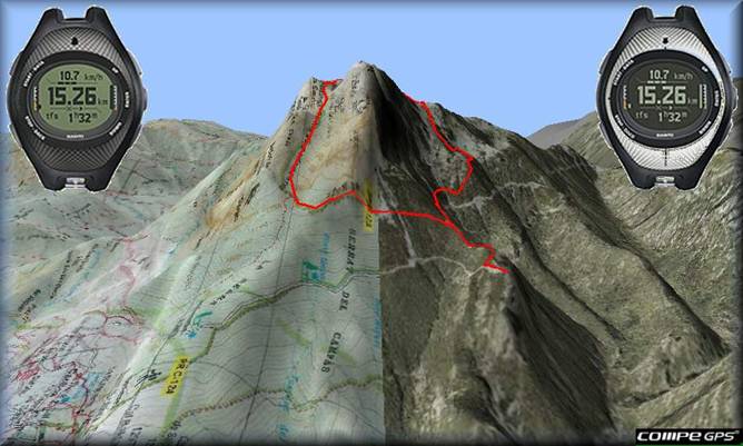
The displaying features of CompeGPS are just great. It is capable to combine altitude, orthographic and topographic data, and allows visualize it together with the track logs in 3D. The image at the front page of this report is created that way.
CompeGPS can even create movies for later playback. To have an idea about these capabilities, you can watch two animations I made from a track log recorded with X9i:
1. 3D animation of a mountain hike (14MB, mpg2)
2. 3D animation of the track log of this mountain hike (21MB, mpg2)
5.1.2
Displaying
Tracks in STM (Suunto Track Manager)
On the Suunto site one can read: “The following maps can be used with Trek
Manager: CompeGPS, Bayo, Fugawi, Topo! National Geographics,
The actual
Suunto Trek Manager I have does not work with internet maps or digital maps.
The only possibility is to use scanned (jpg,
bmp or gif only) images of your printed map. (I think that the phrase has
to start as “The following THIRD PARTY SOFTWARE can be
used DIRECTLY with the X9I WRISTOP: CompeGPS …”)
NOTE: Suunto informed me that it is indeed
correct that STM only accepts jpg, bmp or gif images, but no native digital
maps. They probably have cleaned up
their site accordingly.
If you have no scanned maps yet, then you still
can set up your X9i in STM with the USB snake cable connection.
5.1.2.1 Setting up X9i with STM
After
installing STM and X9i drivers, you can plug in the USB snake cable. When you
then launch STM, and attach your X9i to the snake head, you can set up the X9i
by a click on the ‘Connect to X9’ button. At the lower right STM an X9 settings
window appears, where you can make your modifications (See Figure 28):
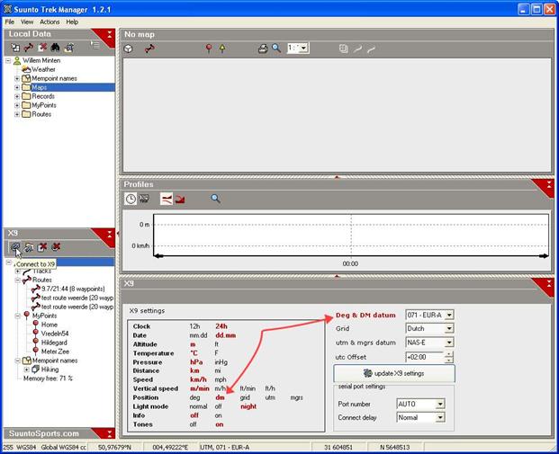
Figure 28 Main STM window and
X9 settings window at the lower right. To the left up the Local Data Tree
window is displayed, to the left down the X9i data memory is displayed.
Note the
relation between the selected Position coordinates, and the pull-down menus to
the right. In Figure 28 ‘dm’ (degrees and decimal minutes) is selected. The
title of the corresponding datum selection set is highlighted. Here the correct datum (071-EUR A) and
Position coordinates dm that apply the topographic map of Figure 7 is selected. This is the setting to update the X9i
with, if you want to correlate the displayed position on the X9i with the map
coordinates (see Figure 9).
If a map
with WGS84 DATUM and UTM coordinates is at your hand, then you can de the
selection as follows:
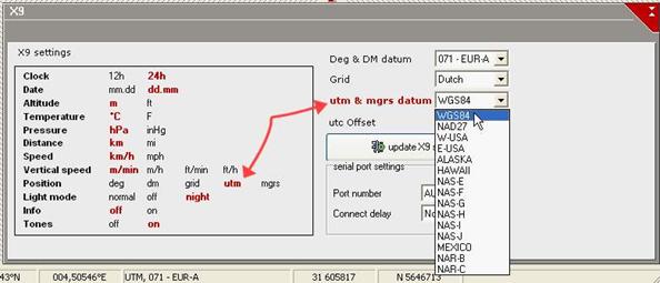
Figure 29 X9i settings window
After
making the selection, the X9i is updated after pressing on the update
X9 setting button.
5.1.2.2 Calibrating a scanned map, and
displaying maps
Calibration
points should be widely spaced.
Assume the
scanned map of Figure 7 is to be calibrated in STM:
First make
STM ready for the calibration of that specific map:
Select one
of the maps in the Local Data window (upper left). Then select your user name
(a direct selection of your name will not show the User settings: this looks
like a bug). The lower right window then looks like this:
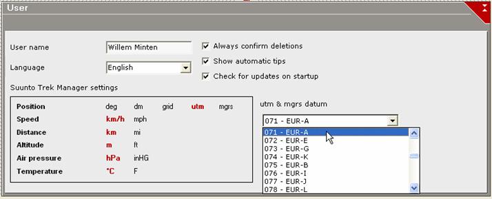
Figure 30 User settings window
STM allows 256 datum’s with UTM coordinates, which is much more than the X9i display can handle (see Section 3.2.2 and Table 4 ). Since the image has a printed UTM grid, it is better to take the UTM position format for the chart calibration. The Datum (071) is assigned as well.
The lower line of the interface gives instant feedback on the position coordinates of the cursor on an imported map:
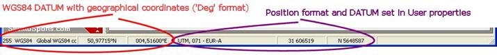
Figure 31 Position coordinates feedback in STM
I noticed the following two map calibration bugs in STM: (1) it is only possible to start a map calibration points in degree based position formats. Adding points in grid based formats causes errors. (2) Another bug concerns the editing of those points. Sometimes it is only possible to edit the grid coordinates while MGRS formats is active (MGRS is just another presentation format of UTM). SUUNTO suggest the following sequence to calibrate:
1. Open the map in calibration mode using degrees format
2. Place two known points into the map so that they appear in different vertical an horizontal level
3. Edit the points locations so that they are "close enough" of the correct values
4.
Save calibration
5.
Then change the user settings
to UTM and try to edit the points.
6.
If this fails, then change to
MGRS and use the "Gridder" application to convert the known UTM
values to wanted MGRS values
7.
Enter the values into
"latitude" column
8.
Save calibration again.
So, after changing the Position format from UTM back to ‘deg’, the scanned map is loaded as follows:
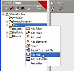
Figure 32 importing a map in STM
After selecting the same map as I used in COMPEGPS, STM warns about the size of the imported map: It has problems with big sized maps with high resolution:
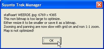
Figure 33 Big sized maps in STM
After accepting, the map is calibrated with two diagonal points containing dummy latitude and longitude (Figure 34 to the left):
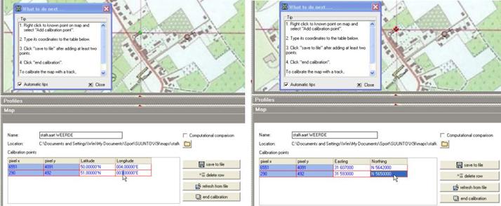
Figure 34 (left) Dummy calibration in degrees, (right) editing the UTM coordinates into correct ones.
Then the calibration is saved, User property Position changed from ‘deg’ to UTM, and calibration is restarted again, to correct for the UTM coordinates (Figure 34 to the right). This is a tedious process. The changing of the UTM coordinates is most easy when the entire field is selected (it takes a few seconds before STM reacts) and edited from first to last digit.
When two diagonal points are calibrated that way, you can save your calibration effort. Then restart the calibration for the third time and try to add supplementary UTM coordinates at different map points. This works for me, but some people need to go back to ‘deg’ position format.
I experienced that the addition of other calibration points does not improve much the quality of the calibration. Only the first two calibration points influence a lot the calibration. I try to catch feedback form SUUNTO on this matter. The following Figure 35 illustrates the effects of this behavior:
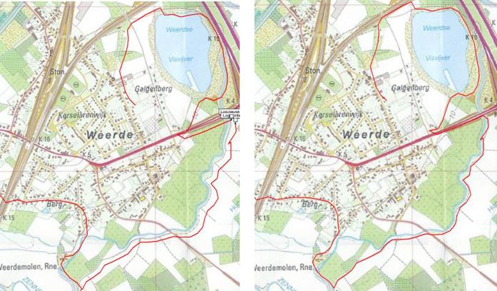
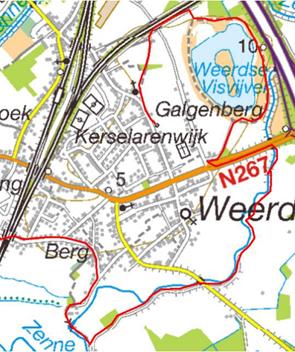
Figure 35 the same track on
the same map (only a small part of the scanned map is displayed), calibrated
with the same 11 points (in the same order). (LEFT) STM, (RIGHT) COMPEGPS. The
difference is remarkable. (BOTTOM) same track log displayed on a full digital
map (NGI topomaps
To obtain the best calibration results in STM, it is extremely important to locate the 2 (diagonal) points close to the Tracks/Routes, and I feel that it is at this time not very useful to use more than two points for the calibration.
This also shows that it is not a good idea to trust blind on the calibration of scanned maps. Some software’s do a good job, others need an improvement. As result, it is not recommended to use scanned maps for the evaluation of the accuracy of the track recording. To do good evaluations, real digital maps with vector components are needed (as it is done in Section 8.2).
To work properly, the map calibration file (extension *.map) has to stay in the same folder as the map image.
To display a map, just select the map reference that already was imported in the database (upper left window. Only one map at a time can be displayed in STM.
Note that also in STM there are other possibilities to calibrate a map. E.g. you can pick-up a track or a few waypoints, and use that to calibrate your scanned map on. When you do that, you just load your track log on the uncalibrated map. Then you can move your map under the track log to match e.g. the starting point. Then you can pick up the end point, and drag it to its correct position. I feel this is a very easy method.
This method however can not ‘prepare’ your trip in advance (Route programming) when you haven’t done such an initial track log recording on the field. Second, the problems discussed above still apply: you will need to catch diagonal begin and end points close to the location of your specific trip.
5.1.2.3 Reading
Once the X9i is connected with STM, Tracks,
Waypoints and Routes can be copied from X9i (middle left window). Choose
appropriate folder names in the STM database (upper left window) to ease future
retrieval. See Figure 28.
The track properties can be edited (like color and thickness) to make them more distinct to other displayed tracks. The upper left part of the Map window serves to hide/display (check mark) or remove (x mark) the track form the current map.
Zoom and pan facilities work fine, as long as the size of the map is relatively small
The merger of two Track logs is not possible yet in
STM. You can do it in GPSBabel (see Section 5.2), which can do the job directly on the sdf export
files (well, almost).
5.2 Digital mapping software without X9i
drivers
5.2.1 Displaying in other software than Google Earth
Assume I
have digital mapping software with vector maps, but the software hasn’t the X9i
drivers for a direct communication with the X9i. Then it would be nice to use the export files
of STM and use it in that other software.
One of the must-have
programs for this purpose is GPSbabel (www.gpsbabel.org ):

Olaf Klein
(http://www.gpsbabel.org/people/olafklein.html
) was very willing to integrate SUUNTO STM files (WayPointPlus files and
SuuntoDataFile) into GPSBabel. At this
time the official release integrates already WayPointPlus files which only
describe the position coordinates of Tracks and Routes. I now am testing a beta that covers
SuuntoDataFile files that describes altitude info and MEMory points as well. In
September I plan to do the last tests for Olaf.
GPSbabel is
command line oriented, but Olaf also wrote a Windows GUI. I’ll use that GUI to
explain how GPSBabel can do many valuable jobs for the X9i.
The
Topographic maps of
Both
softwares can’t communicate with the X9i. I’ll show in the next section how to
do the transfer for the Belgian case.
5.2.1.1 Example: Transcode track logs with
GPSBabel to NGI Digital Topographic Maps
To give an
example how it works, I’ll use the same track log as is used in Figure 35. In STM I
exported this track log as WayPointPlus file.
After
installing GPSBabel (www.gpsbabel.org ),
the GPSBabelGUI looks like this:
In this
interface you need to enter the following items correctly:
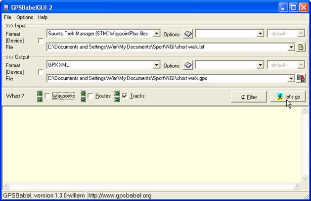
Figure 36 GPSBabelGUI
1.
select
the correct INPUT file format with the pull-down selection arrow (STM WP+ file
format)
2.
then
select the proper WaypointPlus file with the File Open Dialog Button ![]()
3.
Then
select the correct OUTPUT file format with the pull-down selection arrow (GPX
XML file format, which is a general XML format. You might have luck and choose
a specific format for your specific software. GPX is the only one that is
accepted by the software I use)
4.
then
select the proper output location and file name with the File Open
Dialog Button ![]()
5.
at
last ONLY check what is to be transcoded. Here the evident choice (Tracks) is
selected. Other input/output file formats allow different chooses.
When these
5 things are entered in the interface, the button ![]() becomes selectable. Click on it, and the file
is transcoded according to the settings made.
becomes selectable. Click on it, and the file
is transcoded according to the settings made.
Then I can import that GPX formatted track log in the target digital mapping software:
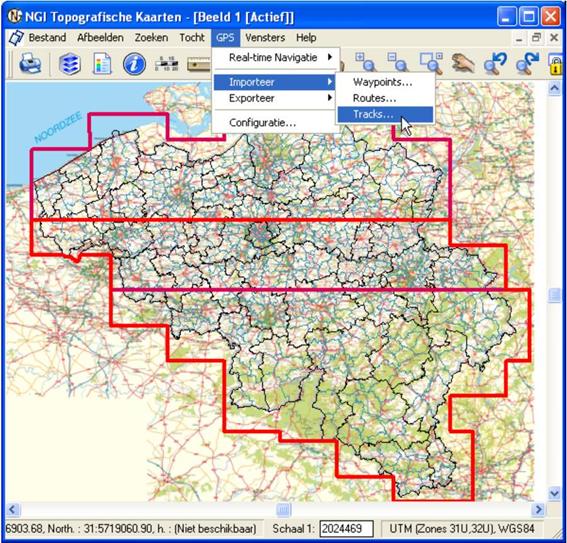
Figure 37 Importing a GPX formatted track in digital mapping software that doesn’t have X9i drivers. (Example http://www.ngi.be/NL/NL1-10.shtm )
The result is given in Figure 38.
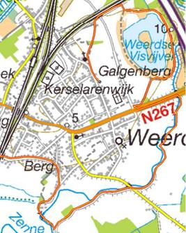
Figure 38 Representation of the X9i track log in a
vector digital map (http://www.ngi.be/NL/NL1-10.shtm ). The track log is transcoded by GPSBabelGUI (www.gpsbabel.org ).
5.2.2 Displaying in GoogleEarth
5.2.2.1 Transcoding to GoogleEarth with GPSVisualizer
You can use
the same method as described above (using GPSBabel) to transcode your track log
to Google Earth. However, for this
purpose I use GPSVisualizer (www.gpsvisualizer.com
):

GPSvisualizer embeds the GPSBabel engine as
well. It is a web application in which
Tracks of any format can be imported and displayed on Google Earth (KML
format): http://www.gpsvisualizer.com/map?form=googleearth
It also has
a online GPSbabel interface that allow you to use that software without
installing it on your hard disk: http://www.gpsvisualizer.com/gpsbabel/
Recently
GPSVisualizer also facilitates working with the X9i as also sdf files can be
transcoded as well! (Thanks Olav and the GPSVisualizer team)
To give an
example how it works, I’ll use the same track log as is used in Figure 35. In STM I exported this track log as an sdf file.
Then you
need to have installed Google Earth from http://earth.google.com/
.
Then
navigate to http://www.gpsvisualizer.com/map?form=googleearth
, and browse to your sdf file as is shown in Figure 39:
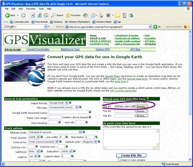
Figure 39 GPSVisualizer interface transcoding X9i sdf files straight into GoogleEarth KML files
Then press the button Create KML File . The result is shown in Figure 40:
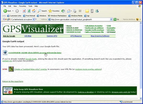
Figure 40 Output form of GPSVisualizer
By clicking on the kmz file, GoogleEarth is launched and the track log is displayed:
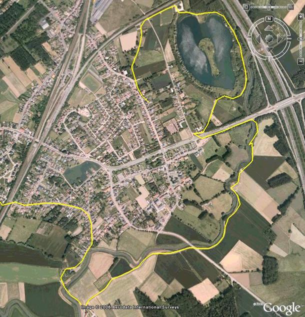
Figure 41 Google Earth representation of the X9i track log, generated by
GPSVisualizer.
5.2.2.2
Transcoding to GoogleEarth with STE (Suunto
Track Exporter)
Suunto Track
Exporter is designed to transcode X9i recorded logs straight into Google Earth.
![]()

STE can
be found here. Google Earth can be found here (http://earth.google.com/).
After
installing STE, X9i drivers and Google Earth, you can plug in the USB snake
cable in a free USB port in the computer
If you start STE when the X9i is attached, it will display all the recorded tracks (Figure 42, right). If you attach the X9i after starting STE, you will need to press the Connect button (Figure 42, left) before STE shows the recorded logs.
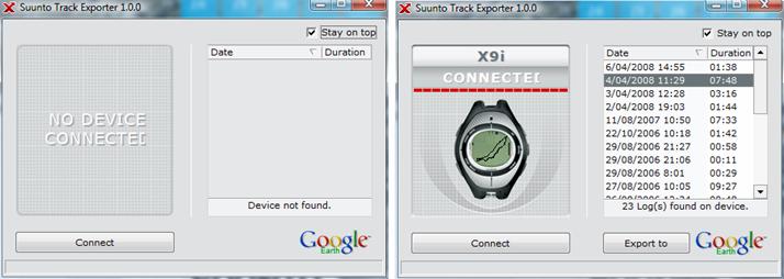
Figure 42 STE Export facility to
Google Earth. Every recorded tracklog is
immediately displayed in the virtual X9i display to the left in STE
Then select
a log to be exported (which will be displayed to the right), and press on the Export to button. Google Earth will start and the
tracklog will be displayed and saved in the ‘Temporary Places’ folder (see Figure 43).
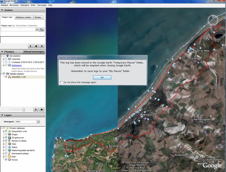
Figure 43 Google Earth
displaying an exported X9i tracklog (North of
To keep the
logs, don’t forget to move them to the ‘My Places’ folder (or they will be lost
after closing Google Earth). In order to delete the tracklog in X9i, they need
to be deleted via STM (see Figure 29, X9i window to the left), or directly in X9i
(Activity window, MEMORY).
5.3 What to do with Google tracks ?
Using STE is an easy way to copy recorded tracklogs to Google Earth. In order to reuse this copied track in other mapping software, the KMZ/KML formatted tracklogs in Google Earth are to be recoded in a useable format. An easy way is to use GPSBabel again.
An example:
Assume a tracklog is exported into Google Earth with STE, and moved it into ‘My places’. Then, by right-clicking on the tracklog, it can be exported as a KML or KMZ file (Figure 44)
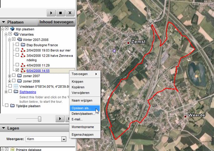
Figure 44 Exporting a track log from Google Earth as a KMZ (zipped) or KML (unzipped) file
Similar to what is explained in Figure 36, GPSBabelGUI can be used to transcode the unzipped KML file (NOT the zipped one) to any other format, here general GPX (
Figure 45):
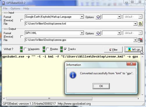
Figure 45 GPSBabelGUI used to transcode a KML formatted track
log to GPX format.
That way one can pass around STM to draw the track log in another mapping software without X9i drivers (example Figure 46):
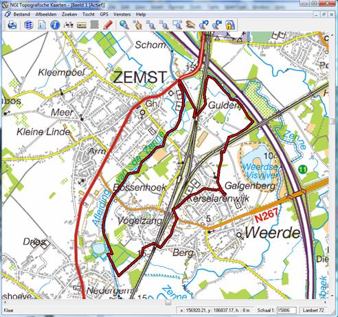
Figure 46 Importing a GPX formatted track stemming from a Google Earth KML track log. (Example http://www.ngi.be/NL/NL1-10.shtm )
The easiest
and most accurate method to program Routes is to work with digital mapping
software with X9i drivers (COMPEGPS, STM, …).
The most accurate method is to use software that can handle vector
digital maps (http://www.ngi.be/NL/NL1-10.shtm,
…), or scanned maps that are calibrated accurately (www.compegps.com ).
This
Chapter assumes that the reader already managed to display tracks in the
specific softwares (see Chapter 5).
6.1 Digital mapping software with X9i
drivers.
6.1.1
Programming
Routes / Individual Waypoints in COMPEGPS
At this
time, the writing of individual Waypoints to X9i is not yet possible. CompeGPS
noticed some problems with the X9i drivers, and is waiting for an answer from
SUUNTO on this matter. For the time
being, GPSBabel can do the transcoding from the WPT formatted file of Waypoints
to a WPP formatted file, ready for import in STM.
The writing
of Routes is processed the similar way as reading a track (described in
previous Section 6.1.1.)
6.1.1.1
Creating
a ROUTE/WAYPOINT
When scanned
maps are used to program Routes and Waypoints, the map has to be calibrated
correctly (See Chapter 5).
In Figure 47 it is shown
how a Route is programmed. By doing a right click on the first Waypoint
location, a pop-up window appears that offers the choice to create a Route or a
singe Waypoint.

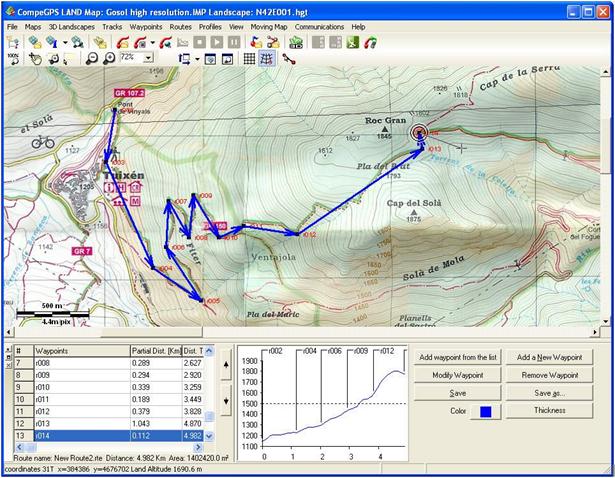
Figure 47 Creation of a Route in COMPEGPS. After the first Waypoint is defined, a ‘Route Editor’ window appears at the bottom. A next waypoint of the route can be appended with the CTRL key: The last new Waypoint is always encircled; by pressing on CTRL, this waypoint shows a hair towards the location of the cursor; by clicking on the left mouse button (while CTRL is pressed), a next Waypoint is created at the position of the cursor. Remark as well the elevation data of the Route. This elevation data is assigned automatically if elevation date of the area is available. The created Route can be stored for future use by saving it as an .rte file. (‘save’ or ‘save as’).
Remark the
elevation data of the Route. CompeGPS allows extracting the altitude from sea
level when a 3D landscape is loaded as well behind a scanned topographic map.
Then the underlying 3D landscape data offers instant altitude information. 3D
landscapes of your scanned and calibrated images can be downloaded from the 3D
landscapes pull down menu. An
alternative is to use maps with altitude information (like Google maps).
The waypoint properties can be edited in a separate ‘Waypoint Editor’ pup-up window ‘double click on a Waypoint in the ‘Route Editor’ window, see Figure 48):
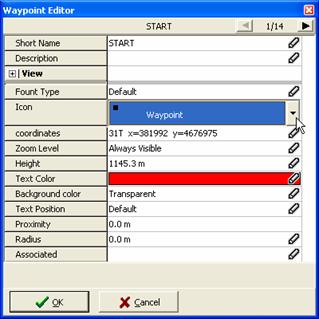
Figure 48 Waypoint Editor. Notice the small arrows on the top right of this window.
The inserting of a waypoint in a Route is
done in the same way as appending a Waypoint. First select the Waypoint after
which a new Waypoint is to be inserted. Then, by using the CTRL key a new
Waypoint can be inserted at the location of the mouse cursor. See Figure 49:
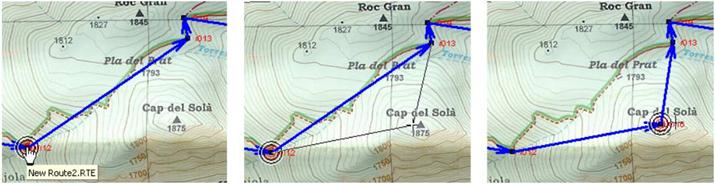
Figure 49 Inserting a Waypoint in a Route.
Moving a Waypoint
can be done by dragging the selected Waypoint to another location.
The
creation of a separate Waypoint can be done in a similar way.
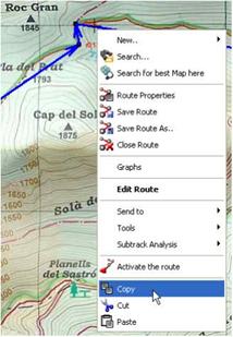
Figure 50 Context menu of a
Route in which additional options can be selected.
Note that
the changes made are not saved automatically. That way, you can easily undo
wrong manipulations by reloading the ‘old’ Route without saving the actual one.
To save the changes done on a Route, you need to select ‘save Route’ or ‘save
Route as’.
To cut
Routes into pieces or concatenate Routes, this saving mechanism is helpful.
6.1.1.2
Writing
the Route to X9i
If you have
installed CompeGPS with the X9i (See Section 5.1.1.1), then it can be uploaded to X9i by selecting
‘Communications’, ‘Send Route to the GPS’.
6.1.2
Programming
Routes / Individual Waypoints in STM
The
creation and editing of Routes in STM happens to be slow and isn’t implemented
in a handy and intuitive way. Moreover, it seems that the used database digests
the changes (even name changes) relatively slow.
It is
important to know that route and waypoint manipulations are executed directly
in the database: there is no need for a confirmation. There is also no ‘undo’
possibility. So, if a waypoint is
deleted accidentally from a route, then this waypoint is to be inserted again
in the route.
In the
sequel I focus on some important manipulations that are not well explained in
the help files.
6.1.2.1
Creating
a Route from scratch
If one has
no calibrated map, then routes can be programmed in the Route window. In this
window one can append new waypoints at the end of route by using the arrow-down
key and entering its coordinates. Be
sure you first have set the correct datum and used coordinate system in the
Suunto Trek Manager settings.
If there is
a calibrated map available (see Section 5.1.2.2), then a route can be created in the map window.
First select/create a folder in the Local Data Tree window, in which the route
is to be stored. Then press on the ‘Route creation button’ (see Figure 51), and start clicking on the map to enter new
Waypoints appending the Route
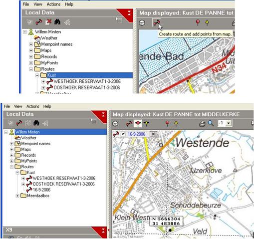
Figure 51 Creation of a new
route in the Map window. First define a folder in which the map is to be
stored. Select this folder, and click on the Route creation button on top of
the map. A default route name is given, and an ‘Add waypoint to created
route’ button is activated. Then every click on the map will add a next
route waypoint.
To move the map without accidentally
creating unwanted waypoints, you can toggle the ‘Add my point button’ in the
map pane tool bar. You
can also press and hold the mouse button down, and drag the map as well
(press and hold the left mouse button will not create a waypoint).
6.1.2.2
Editing/Inserting/Deleting
a Waypoint somewhere in the route
6.1.2.2.1 Editing
It is not
advised to edit a series of waypoints in a track by changing manually
the coordinates in the Route window. I often found that only the changes of the
first waypoint were accepted by the database; all the other changes made on the
next waypoints were overwritten by its original values. This is probably a bug.
Editing one
waypoint will in general pose no problems.
6.1.2.2.2 Inserting
Route window:
In the Route
window (lower right), right click on one of the existing Waypoints of the route
before which you want to add a new Waypoint. Then use one of the options shown
in Figure 52:
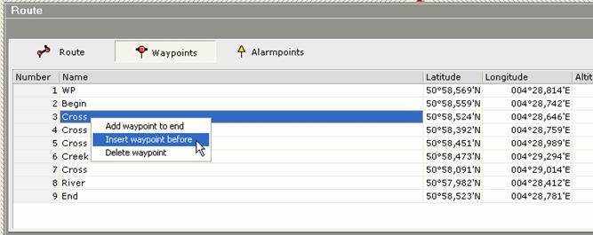
Figure 52 Editing an existing
Route.
An inserted
Waypoint will have the same coordinates as the selected one (also when you
select ‘Add waypoint to end’). You then will have to edit the coordinates in
the Route window, or drag it in the map window. This dragging is tricky because
two points are on top of each other, and you will not know which point you are
dragging. I feel that the waypoint which comes first in the route, is also
selected for the dragging.
Other
waypoint inserts can not be done in the Route window.
Local Data Tree view window:
The Local
Data Tree view window (upper left) offers different facilities to insert
waypoints. After opening a route and displaying its waypoints, one can use the
right mouse button to obtain the following pop-up:
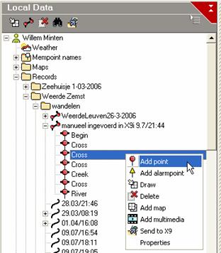
Figure 53 Right mouse click on a waypoint of a route in the Local Data window
By selecting ‘Add point’, a new Waypoint is added as last point in the route. The coordinates of this new waypoint is the same as the one that was selected.
Because this new waypoint is the last in the route, it is hard to select and move it in the map window.
Fortunately there is another option to move the waypoint to another place in the route: this is in the Local Data window itself: Click in Local Data window on the waypoint to be moved, and drag it on top of another waypoint in the same list. Then release the left mouse button, and another pop-up comes on the display:
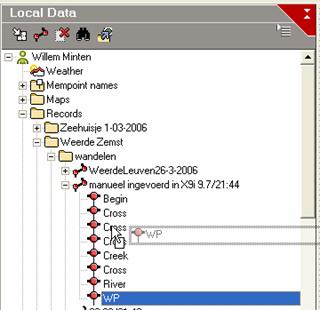
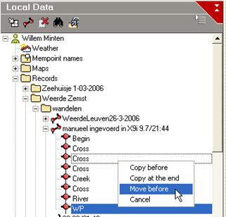
Figure 54 Additional Waypoint manipulations in a Route. The ‘Moving’ of waypoints (changing its sequence) is only possible with waypoints of the same route.
Map
window:
A similar method is available to insert a waypoint from the map (see Figure 55):
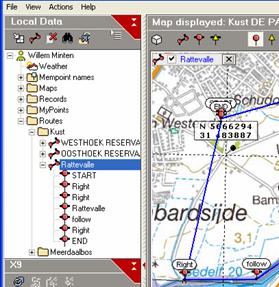
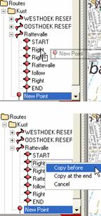
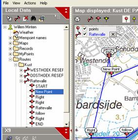
Figure 55 Inserting a new waypoint
with the map window and Local Data Tree view. (LEFT) In the Local Data Window,
open the Route. Then create a waypoint in the Map window by using the ‘Add
points to folder’ button on top of the map. (MIDDLE: TOP and DOWN) Then select that new
waypoint in the Local Data Tree view, and drag it to the waypoint of the route
before which it is to be placed. Then select ‘Copy before’ in the pop-up.
(RIGHT) result of the insert.
Remarks:
1. Except from dragging existing waypoints to a different location, I have found no method that allows modifying routes by using only the map window.
2.
By using the CTRL key one can
select multiple waypoints as well. This is beneficial if one wants to delete a
part of the route without deleting point by point.
6.1.2.3
Splitting
the Route into pieces
This is
useful if one ends up with more than 50 Waypoints (=the Route size limit for
X9i).
Since there
is no split facility, I see two possibilities to do the job:
First possibility:
1. Create a new (blank) route alongside
the route to be split.
2. Copy the route to be split on this
new route (drag and drop the route, and select in the pop up window ‘Copy all
at the End’).
3. open the new route and delete the
first part (use the CTRL key when you select point by point, then press
4. open the original route and delete
the second part in the same way.
There is
however a bug: I often notice that the order of the waypoints in the copied
route (in step 2) is mixed, making this method not effective.
A second possibility is to create two new routes:
1. open the original and first new
route;
2. select by using the CTRL key all the
waypoints of the first part;
3. drag this selection into (not onto)
the first new route, and select ‘Copy all at the End’ in the pop up window;
4. go back to the original route, and
select by using the CTRL key all the waypoints of the second part;
5. drag this selection into (not onto)
the second new route, and select ‘Copy all at the End’ in the pop up window
Also here a
bug appears: Only one of the selected waypoints is copied into the new
routes. This makes the second possibility also ineffective.
As result I
have not found a possibility to split random routes in STM. Copying the
waypoints by dragging them one-by-one is however feasible.
6.1.2.4
Concatenate
two Routes together
To benefit
from past effort, routes are sometimes to be concatenated to create a new
route.
In STM I
think the only possibility is the following:
1. Select the second Route in the Local
Data Tree window;
2. Drag it over the
This does
not work always:
1. the two routes must be close to each
other in the Local Data Tree window. When they are well separated (i.e. when
the Data tree is large), the dragging fails since this window has no auto
scroll feature. By closing the X9i window at the lower left side, additional
space can be made.
2. I often notice that the order of the
waypoints in the appended route (in step 2) is mixed.
As result I
have not found a possibility to concatenate routes in STM. Copying the waypoints by dragging them ‘one
by one’ is however feasible.
Note as
well that merging two Track logs is not possible yet in STM. You can do this in
GPSBabel (see Section 5.2), directly on the sdf export files.
6.2 Digital mapping software without X9i
drivers
To use
digital mapping software without X9i drivers, you can use GPSBabel to transcode
the specific output file of that software to STM readable format (WayPointPlus
or sdf). See Section 5.2 on how this works.
6.3 Direct programming on the X9i
display
Some people
have reported that programming routes directly in X9 makes it hang. I haven’t
had that experience with my X9i. I easily can program Waypoints and Routes on
the display, although this takes more time, and it is impossible to name Route
different than the current time stamp. Also, the Waypoint names are limited to
the Waypoint names stored in X9i.
To have
more freedom for assigning these names, you can create additional ones (or
delete existing ones) in X9i with STM. This goes as follows:
In STM
create an additional MEMpoint group by a right-click on MEMpoint names:
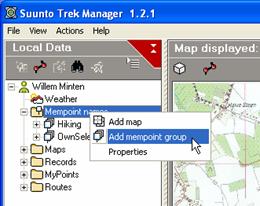
Figure 56 creating a new MEMpoint group
Then add
MEMpoint names in that new group (I take the example of MEMpoint names more useful for cycling):
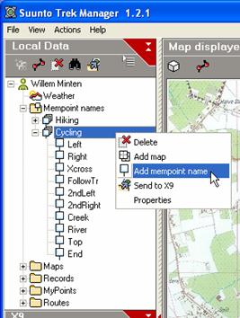
Figure 57 Adding new MEMpoint names
Note that only the first 8 characters of a
MEMpoint name can be displayed. Then upload this group to X9i. Note that X9i
only accepts one MEMpoint group at a time.
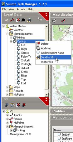
Figure 58 Uploading new MEMpoint names to X9i
Now the Cycling MEMpoints group is available in
X9i.
Be sure you have set correctly your DATUM and
Position or Raster (see Section 3.2.2 or 5.1.2.1), as it is the aim to input coordinates straight from
a map reading.
Then take your X9i and go to the NAVIGATION
DISPLAY MODE, function ROUTE, SUBFUNCTION CREATE.

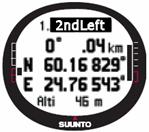
Figure
59 Direct programming of a Route in X9i
The Route name is the creation date,
and can’t be changed in X9i. For the Waypoint
names the current date and time is used as default, but also the Waypoint names
stored in X9i can be selected as well.
The interface in made that way the
editing field has inverse font. To modify the field content, just press ‘Down’
or ‘Up’ (Press-and-hold for faster change). ‘Enter’ accepts the changes made
and jumps to the next field to be edited. ‘Stop/Back’ goes back to the previous
field without accepting the current change. The figure to the right of Figure 59 shows the first Waypoint name is changed into ‘2ndLeft’.
(By choosing such a name, the X9i
user is informed in advance what to do at the next Waypoint.)
When one creates another Waypoint in
the Route, then the initial waypoint coordinates of the new waypoint are these
of the previous waypoint. That way, the changes to be made on the coordinates
are most often small.
Using the ‘Link WP’ SUBMENU, one adds
a new waypoint to the list with the help of an existing waypoint of the current
route. Therefore scroll to that Waypoint
and select it, then select SUBFUNCTION ‘LINK WP’. Linking to a Waypoint of
another Route or to an individual Waypoint in the ‘My Points’ Waypoint list, is
not possible. For these points, one will have to write down the coordinates.
Note that the number of Waypoints in
a Route is limited to 50 (including ALARMpoints), and that the number of Routes
is limited to 25.
6.3.1 Be careful about the map DATUM and
Grid
If one has the ability to use
scanned and calibrated maps or digital maps, then one should use them for the
programming of WAYpoints or Routes.
When one is going abroad for a
journey, often maps become available when one is already on location, i.e.
without the availability of a PC and scanner to digitize the paper map. Then it
is even more important to understand the map compilation notes since the X9i
can not display all kinds of coordinates with all kinds of DATUMS.
The necessity of using a correct map
DATUM and coordinate system is explained in Section 12.3. The following example shows a French topographic map
on scale 1:25000, and tries to identify a useable DATUM and displaying
coordinates for the X9i (Figure 60):
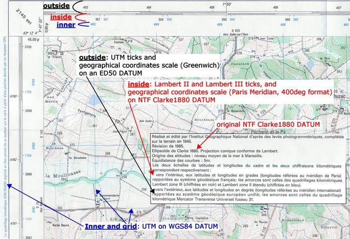
Figure
60 French map showing three DATUMS. This is exceptional. Normally, topographic
maps use coordinates applied to one DATUM, the MAP datum.
The map compilation notes show that three different datums and six coordinate
systems are used:
1.
The
original map DATUM is the ‘Nouvelle Triangularisation de France’ NTF with
ellipsoid Clarke 1880. The original projection system for the map is conic
Lambert III (black numbers at the tick marks at the inside). Also the projection
on cone Lambert II is displayed as blue numbers at the tick marks at the inside).
The longitude and latitude scales on the Clarke 1880 ellipsoid are also given.
2.
At
the outside the UTM
coordinates (tick marks) are given, but not applied on NTF DATUM, but on the
European ED50 DATUM. Also the longitude and latitude scales are given on this
datum ellipsoid.
3.
At
the border of the map it is written in blue that UTM coordinates applied on a
WGS84 DATUM are shown as well at the most inner side. This is as well the grid printed in overlay.
Applying the assignment procedure proposed in
Section 3.2.2.2.2 leads to:
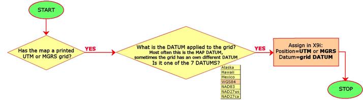
Figure 61 Execution of the
assignment procedure (Section 3.2.2.2.2) to find the Position and Datum to be set in
X9i.
In general, a
‘GPS enabled’ topographic map has an UTM grid. Most of the time however,
the UTM grid is not recalculated towards WGS84 but only towards the original
map DATUM (see Figure 7 and Figure 72). In this case however the UTM grid is related to
WGS84, which is good for the programming of the X9i. After setting the X9i
display to DATUMWGS84 and UTM coordinates, the following map point can be
programmed as waypoint on the X9i display:
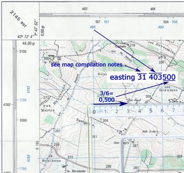
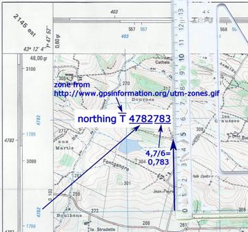
Figure 62 Calculation of the correct
UTM coordinates of a point on the map. The UTM grid shows the kilometers
easting and northing. The fractions calculated by interpolation between the
crosshairs of the grid show the additional meters easting and northing.
6.4
Track
Back
This function is useful if you want to track
back the same track you recorded (so far). Track backs basic idea is to lead
you to the point where you have already been.
With the ‘Track Back’ option, the X9i will
automatically generate successively a new active Waypoint along the current log
or along an already saved log. Track back navigation does not use waypoints of
the normal routes stored in X9i memory, it uses a recorded track log shape and
extracts on-the-fly a next active waypoint on it. This next active waypoint
takes care of the shape of the recorded track log. When there is a long
straight path to follow from the current position, the next active waypoint
will be far away (up to 3,3km ahead I noticed). When the track log shows turns,
the next active waypoint will be close to your current position.
SUUNTO provides me a few examples where this
function is useful. I copy them:
1. You left from your car
and started hiking... in some way of a path you noticed that you have lost your
car keys. At this stage you activate track back, your X9 will navigate you
backwards the same path you just walked. Let’s assume that you found your keys
after few kilometers, if you then change the direction of track back the device
will lead you to that point where you turned around originally.
2. Another hiking example.
You hiked some exciting path in a last month and were very pleased with the
views. On the next month you hiked in the same area and decided to make change
to your original plan and to hike a part of that same exciting route. At this
stage you select that exciting track from last month from your X9i and the
device will lead your to the closest point of that track. When you finally
reach that point then you need to decide which direction you want to re hike
that exciting path und use the track back direction feature.
Starting a Track Back clearly closes your
current track log. Then the X9i starts another log to record from then on your
new positions.
(Most GPS software provides a concatenation
function for track logs. Note also that some GPS software provide as well a
function to generate as well a Route from a track log. That way, I feel it is
better to do the track logging in software because you can judge yourself to
relocate some Waypoints for better navigation.
However, when you are on the field, the ‘Track Back’ comes into play
handy.)
If you do not want to start a new log, then you
can also decide to change your Route navigation into the reverse direction (See
next Chapter) instead of executing a Track Back. This function however does not
work if your track deviates from your Route due to inaccurate navigation or to
few Waypoints. In these cases a ‘Track
Back’ is the only solution to step back on the same track again.
Note that you can not start a track back when
the GPS is not active and there is no log saving process active. So, to track
back a Track log saved in the X9i memory, you will have to do the following:
1.
Activate
the GPS and wait until a fix is made;
2.
Start
a record in Activity Display mode, function Activity ( ► )
3.
In
Activity Display Mode, function Memory, select the Track log to be tracked
back, then select ‘Track Back’.
4.
Choose
‹‹ as the navigation function if you
want to navigate to the starting location. Choose ›› if you want to navigate to the
finish. (see Section 7.1 for the navigation options)
Navigating
with X9i is one of the most easy and powerfull things to do (if you read this
section).
7.1 Navigation options
From a practical point of view, first a programmed Route or Waypoint is activated by using NAVIGATION DISPLAY MODE, function ROUTE. Then you can select the SUBFUNCTION ‘MyPoints’ or scroll down to find your Route.
If you select your Route or individual Waypoint with a long-press on “Enter’, then it will be activated immediately. If you select it with a short press on “Enter’, then you will to press on ‘SELECT’ to activate your choice.
Once a Route or Track is activated, there are several navigation options that rule the automatic navigation on the selected Route or Waypoint (in NAVIGATION DISPLAY MODE, function NAVIGATE):
|
1.
›› means go forward forward to next Waypoint; ‹‹ means go reverse to previous Waypoint, · means go to a specific Waypoint of the Route. 2. A single Waypoint is activated from the list of ‘MyPoints’ Waypoints: ¸ means navigate to this waypoint; (You can’t select this last navigation function is you have activated a Route) There is also one possibility to navigate on, without selecting a stored Route or Waypoint Ï means navigate to the
position where you activated this navigation method. This last method is only useful if you have no Waypoints or Routes stored. |
There is however one possibility to create
instantly (i.e. an instant GPS position during your trip) a Waypoint that will
be accessible right away to navigate on. This is the function
These
symbols are also visible on the lower line in the Navigation display.
Apart from the
normal Waypoints in a Route, STM also allows to program ‘ALARMpoints’ with a
certain Radius within a Route. The X9i
will beep when the current position is within the alarm radius of the ALARMpoint.
They are not used to navigate on, but inform the X9i user for danger like
cliffs.
To make a
distinction between Waypoints and Alarmpoints, the X9i will display them in its
memory with a different icon: ˜ for Waypoints, § for Alarmpoints. Data of the current Route or
individual selected Waypoint can be observed by a press on START/DATA in
Navigation Display Mode.
7.2 The Navigation Display
Besides the
Navigation method, there are other data visible in the navigation display
(assume the GPS is on):
§
On
the top row the name of the active Waypoint, used for the current
navigation, is displayed
§
The
middle row shows the distance from the current position to the active
Waypoint.
§
The
bottom row can display 7 different navigation data figures. The one that
is to be displayed can be assigned in NAVIGATION DISPLAY MODE, function NAVIDATA.
Select one of these for displaying:
1.
dtf : distance to finish. Displays the distance from the current
location to the last waypoint (via each waypoint).
2.
ttw: time to waypoint: Displays the estimated travel time to the next waypoint based on the
current speed.
3.
eta: estimated time of arrival: Displays the estimate arrival time to
the last waypoint based on the current speed.
4.
ete: estimated time enroute: Displays the estimated travel time to the
last waypoint on the route, based on the current speed.
5.
atf: altitude to finish: Displays the total amount of ascent from the
current location to the last waypoint in the unit of your choice.
6.
spd: speed: Displays the speed in the unit of
your choice.
7.
hea: heading: Displays the heading in degrees
8.
Xte: Cross Track Error: (Left or Right) This is the shortest distance (to the
left or to the right) from your current location to the straight line connecting
the previous and next Waypoint of the route.
In my X9i am missing Navidata number 5. Probably
replaced by 8 (which turns out to be much more valuable during navigation). In any case, it would be impossible for my
X9i to find the atf, since the
waypoints in X9i don’t display their altitudes.
On the
missing atf, Suuntosports member
Roberto says: “…on section 3.5.3 of
Suunto X9i manual ‘creating a new route’ it is shown the altitude field,
whereas in my X9i I can not see it excepting if choose the option of “update”
the waypoint being the GPS on. By the way when I download a route to the
computer either by STM or by compeGPS I got the altitude field with the right
values, therefore the altitude filed must be somewhere in my X9i but I can’t
see it, which it is a bug...”
There are
also other navigation displays that show information about the current selected
route. These can be accessed with
‘START/DATA’ button from within the NAVIGATION DISPLAY MODE (only when a
Route is activated). The ‘UP’ and ‘DOWN’ buttons are used to display all the
data of the Route Waypoints. The data displayed depends on the selected Route
navigation method (›› , ‹‹ or · ).
The X9i
automatically reports the bearing and distance to the next Waypoint (with a
circular bearing indicator ˜ at the edge of the display). And if the
current speed is not sufficient to trace the bearing with GPS, then the electronic
compass takes over automatically (with a circular bearing indicator š at the edge of the display. This
feature however only works with a GPSFIX=1sec. When the GPSFIX=1min or manual,
the circular bearing indicator of the compass is not available in the
navigation window. I think this is a bug.
In the
following Figure 63 a navigation to the single Waypoint Home is displayed
at the time the GPS signal reception was perfect (5 bars), but the electronic
compass has taken over the navigation direction. This means that the X9i user
stood still and the GPS receiver was unable to trace the correct direction to
the Waypoint Home.
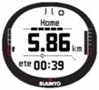
Figure 63 Automated hybrid GPS–ElectronicCompass
navigation with X9i.
In normal
route navigation, the unit automatically switches to the next waypoint when you
arrive inside a 30-meter radius of the waypoint or pass it at a distance
further than 100 meters of the perpendicular line to the route that goes
through the waypoint.
Note that
the direction of travel to the next Waypoint is related to the fixed sighting
marks. Depending on when the GPS is used or the electronic compass is used. See
Figure 64:
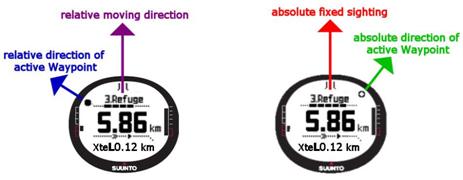
Figure 64 Visualisation of
the direction to the next Waypoint with a GPS and compass bearing indicator.
The fixed sighting marks û ë are understood either as the relative instant direction of travel
found by GPS, or as the absolute direction in which the X9i is directed
instantly in the horizontal plane. The
displays show an optimal GPS reception (4 to 5 bars). In the figure to the left
the X9i detects a speed that is sufficient to trace the relative direction of
the active Waypoint. In the figure to the right the X9i does not detect a
sufficient high speed, and the compass takes over and shows the relative direction
of the active Waypoint.
Hence, the
position of the GPS bearing indicator ˜ is independent of the direction in
which the X9i is held in the horizontal plane. This is not the case for the
compass bearing indicator š.
Note again
that in the navigation window, the compass circular bearing indicator š is only available when the GPSFIX=1sec. When
the GPSFIX is 1min or manual and the GPS is active, the only possibility to
navigate on when the GPSbearing indicator ˜ is not available, is to select the Compass
Display and navigate on the current bearing (Thanks to Suuntosports member Colin).
7.3 Compass display mode
Prior to
your trip, you should set correctly the two following functions in Compass
Display Mode:
1. Calibrate the compass prior to a long
trip (or during the trip when you experience it is disturbed). I haven’t found
a sudden disturbance when my trips are outside of urban regions.
2. Set correctly the declination:
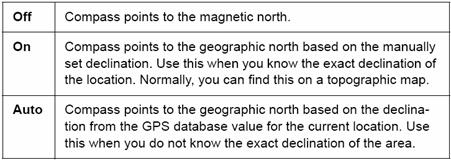
Table 6 set up of declination of the X9i electronic compass
The main window looks like

Figure 65 Main Compass window. The third line is set to display the compass bearing. For this setting (only), the display shows the fixed sighting marks û ë (pointing to the direction the X9i display is set) at the top of the edge, and around the edge the display shows a hollow North indicator š (pointing to the North). If the X9i is pointing to the North, the top of the edge will show ûšë
The main display has three rows, and at the edge the circular North indicator:
§ The first row displays the cardinal and half-cardinal point abbreviations.
§ The second row displays the heading in degrees.
§ The third row can be set by selecting STOP/BACK:
o the current time,
o the bearing lock (L or R), which helps you follow a certain bearing.
The lock is set as follows: Rotate your Suunto X9i horizontally until the desired bearing is displayed on the second row. Then, while the compass is active, press START/DATA to select a new target bearing.
The bottom row displays the degree deviation, to the left or right, from the target bearing.
o Bearing (bea):
§ If you are navigating a route from the Navigation menu, the third shortcut displays the bearing to the next waypoint.
§ If you have not activated a route and the GPS is on, the shortcut displays the bearing to the start position (where the GPS or an activity was switched on). If the GPS is not on, the shortcut displays the latest acquired bearing.
Figure 65 shows the X9i display in COMPASS MODE while the third
line is set to show bea.
Because the
X9i is made as a wristop GPS which needs a fluent operation in all positions,
it is designed with a build-in loop antenna. Such antenna types have a wide
radiation pattern, which receives data from a wide angle. However, due to the wide angle, the
sensitivity of reception is not as good as in hand-held GPS receivers with build
in or external narrow radiation pattern (typically patch antennas).
8.1 Precautions
To get the
most accurate GPS readouts, take care of the following:
1.
Before
starting a navigation/record:
a.
Establish
correctly an initial GPS FIX when the X9i is unaware of the actual satellite constellation
(See Section 3.3). If you do an initial FIX, then wait at least 15
minutes after the first FIS has been established. To minimize the GPS
initiation time, hold the unit steady (off the wrist) in one position with the display
facing up and make sure you are located in an open area so that the unit has a clear
view to the sky.
b.
Operate
at the start of a GPS FIX in a similar condition as with an initial FIX. I.e.
i.
Do
not move the X9i (don’t hold it on your wrist but place it somewhere on a safe
spot with clear sky conditions;
ii.
The
signal strength reception must be at least three bars, preferably 4 or 5 bars
iii.
Make
a GPSFIX with at least 6 satellites (generally within 60 seconds), and wait
until the epe is evolved to be smaller than 1 meter (another 30 seconds).
During the
trip:
1.
if
you are in a team, do not let the team
members walk along the X9i, but let your wrist be on the free hand with clear
view on the sky;
2.
Avoid
coverage of (wet) clothes, but use the extension strap and wear the X9i outside
your clothes.
There are
of course unavoidable obstacles during the trip. Therefore it is advised not to
use the GPS receiver in extremely bad reception conditions (like dense tree
coverage on a rainy day), to save battery lifetime.
8.2 Three illustrative examples
This
Section shows some typical examples that illustrate the overall quality of the
GPS reception of the X9i.
The
equipment used for the first two comparisons was the following:
Ø X9i set on GPSFIX 1 sec;
Ø STM to download the track log from
X9i and export the track log as Waypoint Plus file;
Ø GPSBABEL (www.gpsbabel.org ) used to transcode the Waypoint
Plus file to a universal GPX format;
Ø Digital Mapping Software http://www.ngi.be/NL/NL1-10.shtm of
the National Cartographic Institute of Belgium that reads GPX formatted track
logs, and is capable to establish a mapping of the track log onto a true
digital map. (See Section 5.2.1.1 how the transcoding has been done). Consequently, the comparisons are made on true
digital map data on scale 1:10.000, and not on scanned and calibrated maps.
This is a necessity to do accurate track log comparisons, as it is already
proven in Figure 35.
This set-up
allows having a good interpretation of the accuracy of the recording process,
which depends on the quality of the correlation process of the GPS signals.
8.2.1
Demanding
example
Track log of a GPS demanding hike in a dense
wood on a cloudy and rainy day. Supplementary, the GPS FIX was not done in
ideal conditions (only a FIX of 4 satellites was established and the signal
strength reception was only 3 bars strong).
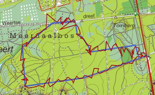
Figure 66 A GPS demanding hike in a dense wood on a cloudy rainy day...
The blue path show the
true track hiked (ROUTE). The red path shows the recorded TRACK LOG. During the
hike the signal strength reception is varying between one to three bars (never more
than 3 bars). The X9i even looses once in a while all satellites (blinking signal
strength indicator). The distance of the ROUTE is 6,42km; the distance of the
TRACK LOG is 12,08km.
This example shows
that it seems better to do a manual GPSFIX at certain points of the ROUTE (or a
1min GPSFIX) where the density of the trees allow for a relatively well satellite
reception.
8.2.2 A less demanding example
Track log of a cycling tour. X9i attached on
the handle bar. The GPS fix was fine, and the ROUTE was of mixed behavior (from
clear sky conditions over normal foliage to narrow streets in some towns). During the trip, the signal strength always
was from 3 to 5 bars.
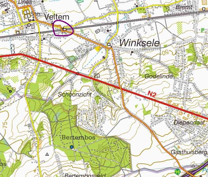
Figure 67 Bike trip. The track log is
depicted as a red-yellow
colored path. Only a small part of the track log is
displayed.
The whole track log shows a perfect match with the streets of the digital map. I only have seen one small irregularity in the whole track log (30 km ride) where I used a pedestrian tunnel going under a railway and the GPS looses all satellites for the time being under the railway (this location is encircled in purple).
Other experiments show similar results. I conclude that the (small) X9i performs similar to the regular (handheld) GPS tools: it works perfect in ideal conditions, but can show a performance breakdown in demanding conditions of operation.
8.2.3
A
best practice example for demanding conditions
The GPS
demanding hike/climb was done at the Pedraforca, a well known steep Catalonian
(
CompeGPS (see
section 5.1.1) is used for downloading the track and displaying it on
a 3D chart with elevation data. The downloaded map was ‘Catalunya Ortho 1:5000’
from ICC (thanks to Institut Cartogràfic de Catalunya), the elevation data downloaded was downloaded from
The first
part of the journey (half way the top) was done with GPSFIX 1 sec. The second part of the journey (up to the top) was
done with GPSFIX 1 min. Both parts
have a red colored track log. The third part of the journey was done with a manual GPSFIX: when the view to the satellites
allow, a manual fix had been executed. This part of the track log is colored in
blue.
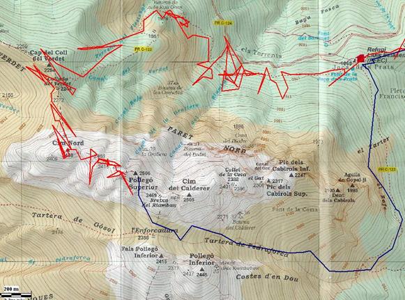
Figure 68 Track log recording in demanding conditions. Everywhere the track
is under trees or very close to tall rocks. When the GPS signal strength is
weak, it is better not to use 1sec GPSfix. When the GPSsignal strength is very
weak, it is even better to do a manual GPSfix.
The
conclusion of these three examples is that if the GPS reception is continuously
strong (3 black blocks or more) then a GPSFIX 1 sec offers the best results. In
demanding conditions however with poor GPS signal strength it is better to
track logs with a GPSFIX 1 minute or even manual.
Note that
good GPS software like CompeGPS allow cleaning up the track log by editing
inaccurate track points.
8.3 Which distance is the most accurate
one?
From the
previous example it is clear that the accuracy of the measured elapsed distance
depends on a proper choice of the GPSFIX, which is related to the view to the
sky and the shape of the track.
If the view
to the sky is good, then a GPXFIX of 1sec can be used, and ideally each 10sec a
track point is recorded. The reconstruction of the elapsed distance from these track
points in GPS software is always an approximation of the elapsed distance
updated instantly in X9i. This elapsed track distance is displayed in the
ACTIVITY DISPLAY MODE and recorded separately in the track header when the log
is closed.
Conclusions:
1. in demanding conditions, it is
better not to use GPSFIX 1 sec. Then the distance found with the recorded track
points are the most accurate ones: when the quality of the GPSFIX is not
sufficient to record a track point, the elapsed distance will be updated
already.
2. When the signal strength shows
continuously at least 3 black blocks, then the elapsed distance updated in X9i with
a GPSFIX 1 sec is the most accurate one.
This
section explains how to make a cheap (€10,00 to €15.00), versatile (for
charging in cars or with different sorts of small sized batteries), compact and
lightweight USB charging device for the X9i.
9.1 Shoping
list
1.
Soldering material (or use press connectors![]() ), and
isolation tape (or use heat shrinkable tube).
), and
isolation tape (or use heat shrinkable tube).
2.
Two sets of 9V (E-block) battery cell snaps![]() . Bought
at http://www.capitani.be/ (an electronic products shop that sell
battery holders and accessories), for €0,3 each.
. Bought
at http://www.capitani.be/ (an electronic products shop that sell
battery holders and accessories), for €0,3 each.
3.
Two sets of  (optional).
Bought at http://www.capitani.be/ , for €1 each.
(optional).
Bought at http://www.capitani.be/ , for €1 each.
4.
A car cigarette lighter female plug. I
bought a complete extension cable  , and only used the female connector, at http://www.auto5.be/ , for €3,99.
5.
A car cigarette lighter USB charger  (10 to 32 Volt in, 5,6Volt 700mA out (max)). Bought in the excellent e-bay shop of Ben http://stores.benl.ebay.be/World-Wide-Magic for €3,50 + €2,70 deliveries. He sells this DC-USB adapter extremely cheap.
I received it within 2 days.
(10 to 32 Volt in, 5,6Volt 700mA out (max)). Bought in the excellent e-bay shop of Ben http://stores.benl.ebay.be/World-Wide-Magic for €3,50 + €2,70 deliveries. He sells this DC-USB adapter extremely cheap.
I received it within 2 days.
The input voltage range is important: these specifications allow charging your X9i with:
a. 8 1,5Volt AA batteries in series, making 12 Volt input at maximum. This is a high capacity solution (alkalines have a typical 2500mAh). In order to charge your X9i when the batteries are not totally fresh, the USB charger will have to allow input voltages as low as 10 Volts.
b. 2 9Volt E-block batteries in series, making 18 Volt input. This is a low capacity solution (alkalines have a typical 500mAh). In order to work, the USB charger will have to allow input voltages as high as 20 Volts.
c. A car or truck cigarette lighter.
There is a LED at the back side that goes off when the charging voltage is below 10 Volt.
6.
A USB extension cable  . I used one from a broken USB 1.1. device. If
you don’t have one, you can find it at stores that sell computer material (for
around €2,00).
. I used one from a broken USB 1.1. device. If
you don’t have one, you can find it at stores that sell computer material (for
around €2,00).
9.2 Assembly
Figure
shows how to make this.
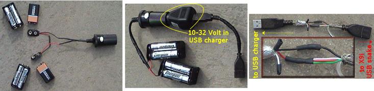
Figure 69 On the field USB charger for the X9i.
Left:
The battery snaps
are soldered in series (+ of one snap (red wire) connected to the – of the
other snap (black wire).
The other two
wires of the snaps are connected to the car cigarette lighter female plug as
follows: The remaining red wire (+ side
of the assembled battery kit) is connected to the wire of the center part of
the plug. The remaining black wire (- side of the assembled battery kit) is connected
to the wire of the can part (outer part)
of the plug.
Middle:
The 10 to 32
Volt DC to USB adapter
Right:
When atttached to
the mains outlet, the tail (USB male) and head of the snake shows the following
voltages at the pins:
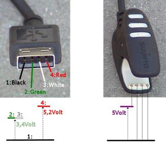
Figure 70 Voltages at the
pins of the USB output of the mains outlet and at the snake. The correct
voltages to charge the X9i are given in the image to the right: the three
rightmost pins do not show a voltage difference, the leftmost pin shows 5V with
respect to the other pins.
For standard USB
contacts, pin 1 is the ground (black wire), pin 4 the +5Volt (red wire), and
pin 2 and 3 are data (green and white wire).
General USB chargers do not provide 3,5Volt at pin 2 and 3. As result,
the USB snake head pins will in general not show the correct voltages when this
snake cable is used with other USB charging devices than the SUUNTO USB mains
charger.
To charge the X9i
with the USB snake cable, the voltages shown in the image to the right of Figure 70 are necessary.
If these voltages are not observed when the snake cable is in operation
with the on the field charger, then this is most likely due to missing voltages
at the data pins 2 and 3 of the charger.
In that case, an additional USB extention cable can be used to create a
positive voltage at pin 2 and 3 as well. In the image to the right of Figure 69 this is shown:
§
At
the side of the USB charger, the datapins 2 and 3 are isolated;
§
At
the side of the snake cable, the datapins 2 and 3 and the pin 4 are connected
to pin 4 of the USB charger;
§
Pin
one of both sides are connected with each other.
With this, the
snake cable USB connector wil observe a positive voltage as well at pin 2 and 3
(no 3,4Volt but 5Volt).
Warning: Before pluging the snake onto the
X9i, be sure that the snake pins show
the same voltages as when it is used with the SUUNTO mains outlet USB charger.
Figure 71 shows the charger equipped with 2 9Volt batteries in
full operation.
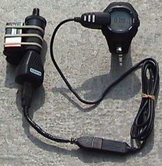
Figure 71 Self made on the field charger of the X9i. The full charging time takes about the same time as with the mains outlet (approx. 6 hours). I experienced that two 9V batteries can do 1,5 times a full charge. To save battery power when the X9i is not charging, the cigarette lighter USB charger can be detached. The 1,5V setup can charge 4,5 times.
9.3 Which battery pack is the best?
See http://www.duracell.com/oem/Pdf/others/ATB-5.pdf
.
The benefit
of the 9V solution is its smallest size, weight (around 95gr versus 220gr
including battery holders) and price (€12,5 per 2 vs.; €16,00 per 8).
The benefit
of the 1,5V solution is its bigger capacity (typical 2500mAh vs. 500mAh).
I found
that the 9V solution can charge the X9i around 1,5 times, which makes me think
that the drain is around 60mA. This suggests that the 1,5V solution should last
2500mAh/60mA=40 hours, which is the equivalent of almost 7 times charging. So
far I managed to charge the X9i around 4,5 times with the same 8x1,5V AA
battery pack.
You can use
as well 10 or 12 1,5V AA batteries instead of 8 (by using as well 6pack battery
holder(s) with snap terminals). If the
battery remaining voltage goes from 1,5V down to 1,1V or even lower, there still
will be sufficient voltage for the USB charger to do the charging job.
Additional weight is the compromise.
Conclusion on the battery pack: if you need to charge more than
one time, then use the 1,5V solution. If you only need to charge 1 time and weight
matters, then use the 9V solution.
9.4 Effects of degraded charging
When the
battery pack remaining capacity becomes low, you can see the following effects
on the X9i display:
§
Black
blocks at the right side stop scrolling, although not all blocks are black.
§
The
last two black blocks keep scrolling for long time without the addition of
another fixed black block
§
‘PC
connection’ comes on the display (with the 9V solution)
|
DISCLAIMER: I do not take any responsibility
when your X9i gets damaged. |
9.5 Alternatives; but watch out.
On the market there are solar chargers. They have the drawback that the chargng is only possible during a clear day while keeping the solar elements to the sky. In late evening or during the night they are unuseable.
There are also other kinds of USB chargers. I have tested a few, and they don’t work because these haven’t accounted for the specific wire connections of the USB snake cable (Figure 70).
Note also that it is wrong to assume that a full charged X9i can guide you throughout the whole journey of one day:
· Even with a 1 minute GPSFIX, it can take a long time before a real fix is made (mountain climbing, tall obstacles, heavy tree coverage). This is battery consuming.
· When the GPSFIX is set to 1 minute, only the GPS bearing indicator is available during the FIX event, and this only when there is a relative moving direction detected by the GPS. If this relative moving direction is not clear for the GPS, and one needs to navigate to the active Waypoint, the GPSFIX is to be set to 1 sec in order to make the Compass bearing navigation available as well (Figure 64).
· In general, ‘navigating’ is much more power consuming than ‘track log recording’.
Knowing this, it should be clear that the following battery lifetime can be estimated as:
|
GPSFIX |
Recording rate for distance |
|
Recording rate for altitude |
Memory capacity (MAX. 24 LOGBOOKS) |
|
1 sec |
10 sec or longer depending on true FIX |
4.5 hours or shorter depending on FIX power |
10 sec |
24 hours |
|
1 min |
1 minute or longer depending on true FIX |
12 hours or shorter depending on elapsed FIX time |
20 sec |
125 hours |
|
manual |
When manual FIX is established |
unknown |
60 sec |
400 hours (around) |
|
no |
no |
2-5 months |
no |
none |
Table 7 Typical recording numbers for X9i
This chapter explains how to use the X9i
for a true journey, when you don’t have a computer with scanned or digital maps
at hand. A journey to the Puigmal located in the northern of
At home I already programmed a few other waypoint names in X9i (see Section 6.3), fit for use in the region where I planned my journeys.
10.1
Preparation
of the hike: creation of the route
A few days before this hike I bought in a local bookstore a topographic map of the region of the Puigmal. To avoid mistakes in programming the route, I observe carefully the map compilation notes, see Figure 72:
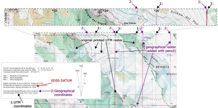
Figure 72 Map compilation notes and grid detection of the topographic map
The assignment procedure for X9i for
Position and Datum is similar as the one depicted in Figure 8 of Section 3.2.2.3: Due to the ED50 datum (widely used in
After carefully drawing these crosshairs manually on the relevant part of the printed map, I am able to calculate the correct latitude and longitude (in the ED50 datum) for a few waypoints along the route, see Figure 73:
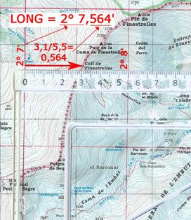
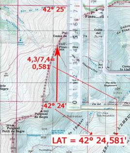
Figure 73 Finding the correct longitude and latitude (in datum ED50) of a waypoint on a map with a manually added geographic grid (red grid). The original printed grid is UTM (black grid), which can’t be used to find the correct coordinates to be programmed on the X9i display. In X9i, the format of the position coordinates is set to ‘dm’ (degrees and decimal minutes). That way, the fraction of the position of the waypoint between the crosshairs of the minutes can be used immediately to enter the decimal fraction of the minutes.
To start the programming, I navigate to the Activity Display menu and select the Route subfunction. The first line shows the memory free. I already did most of the planned hikes, and I see I still have 53% free. So there is no problem to record tomorrow another hike.
It is good to keep track of the programmed waypoints on a sketch or on the map. That way it will be easier to navigate to a single waypoint in the route (occasionally). See Figure 74:
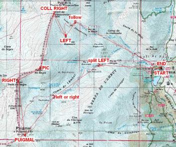
Figure 74 Copy of the programmed route. The numbers and labels are valuable if one suddenly wants to navigate directly to a specific waypoint of the route.
After programming the route, I activate the route. (Navigation Display, Route, long press on ENTER when the route is highlighted). With this, the route name is displayed on the top line of the Navigation display. The middle line shows the route distance calculated from waypoint to waypoint: 10,19km. I have programmed the waypoints that way I also have a good (but slight under-)estimation of the hike distance. The topographic map shows a total elevation of 1000 meters. The hike won’t be a long tough one, so I decide to take my camera with. I believe I will have the opportunity to take some beautiful pictures, since my X9i weather station indicates a raise of the air pressure at sea level during the last 48 hours (upper and middle line of ALTI/BARO in USE BARO mode).
I also set the NAVIGATE option to ››. This starts the navigation of the route from waypoint number 1.
Because I want to reach the top at
This finishes my preparations.
10.2 Executing the hike
At the start location, I first calibrate the electronic compass and set the altitude according the topographic map. I place the X9i somewhere with a big clear view to the sky and let the GPS receiver find a fix with a GPSFIX 1 sec. As soon as a fix is made, the navigation window changes its content. The first line shows the active waypoint (in this case the first one of the active route); the second line displays the distance from the current position to the active waypoint.
To be sure that the X9i starts in optimal conditions, I wait another 5 minutes after the X9i has found a first fix. That way the X9i traces back fast the lost satellites during the hike.
Then I put the X9i on at my right hand side, which will make the display of the X9i oriented towards the valley. This is beneficial for an optimal reception.
Then I start the record of the track log, and start the hike to the first waypoint. The signal strength stays on 3 to 4 blocks, but I decide to set the GPSFIX to 1 minute, which is sufficient to record a low speed hike in the mountains.
I see that the battery indicator shows only two blocks; I forgot to charge the battery the evening before. I take my on the field charging kit, and let the snake cable charge the X9i while it is navigating and recording. This self made charging kit helped me already a lot: I haven’t seen a mains outlet for 5 days during which I used the X9i GPS receiver intensively.
After passing the first waypoint, the second waypoint is activated automatically. I notice an information board saying that, for a better panoramic view, it is advised to do the hike the other way around. I decide to follow that advice, and change the navigation direction from ›› to ‹‹ . By changing this navigation direction, the first waypoint becomes active again. While in NAVIGATION DISPLAY, I press on START/DATA. I scroll from waypoint 1 to waypoint 9 (See Figure 74) and press on ENTER. That way, waypoint 9 is activated; and the X9i will lead me in reverse direction to the original start point 1.
For hiking, my preferred navigation and activity display mode are the ones showing the cross track error and altitude, see Figure 75:
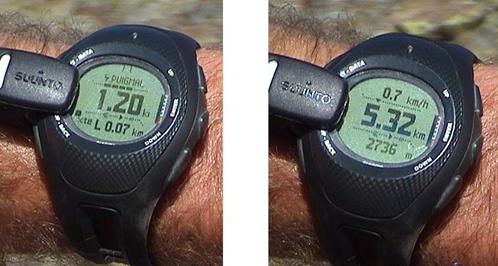
Figure 75 My personal preferences for the lower line of the Navigation and Activity Display: Cross track error Xte and altitude.
As long as Xte is low I know that I am not much separated from the programmed route.
At the top, I first take a MEMPOINT record of the spot. instead of pausing the log record, I set the GPSFIX to manual. With this, the altitude measurements still will be recorded (changes are due to the barometric drift). I prefer doing this because some GPS software’s have problems to interpret such a pause in the track log. STM will make no problems (it even displays activity and pausing times). CompeGPS will ask to unify the recorded log (If negative, then the recorded track log is split at each pause).
I stay an hour at the summit, to enjoy the panoramic view and to eat and drink a bit. I decide to attach my X9i in the shadow to my backpack. I guess it is around 15°C but the radiation of the sun at 3000 meters, and no wind, make it feels like a warm summer day.
After 4h45min I arrive back at the start, the elapsed linear distance report on the Activity window shows 11,43km.
10.3 Post journey analysis
Back home, I upload the track log to CompeGPS. CompeGPS report the distance with height as 13,42km.
I download altitude and orthographic information of the area. The altitude graph looks nice:
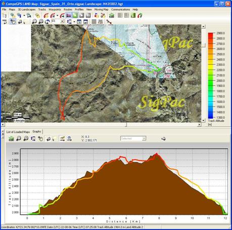
Figure 76 The barometric measured altitude (graph line) on top of the Digital Elevation data SRTM 90mx90m resolution.
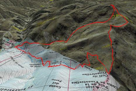
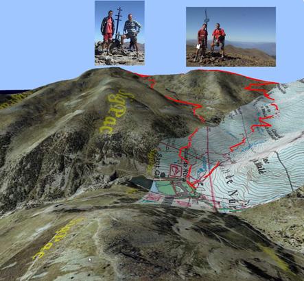
Figure 77 3D views of the hike obtained in CompeGPS, which found
SigPac orthographic maps of
11.1
Firmware
bugs, abnormal behavior in X9i
1. The more WAYPOINTS are programmed in a ROUTE, the more time it takes to accept the next programmed WAYPOINT (‘WAYPOINT STORED’ on display can take a few or more seconds –be patient-). In rare occasions, the display ‘WAYPOINT STORED’ gets frozen.
Workaround: press a few times on STOP/BACK; then navigate to the incomplete ROUTE, select it and add the next WAYPOINT.
2. When using GPSFIX MANUAL while recording a track log (ACTIVITY ►), it can happen that the GPSFIX empty box disappears all of a sudden from the display. When this occurs, it is impossible to set the GPSFIX to 1min or 1 sec: the GPS receiver will not restart any more.
Workaround: set ACTIVITY record in PAUSE (▌▌). Then set it again to START (►). Eventually redo this more than one time with a different GPSFIX setting (1sec). All of a sudden you will see the GPSFIX icon bumping up again on the display.
Beware: do not select ACTIVITY STOP (■), since this will close your current log.
3. ACTIVITY DISPLAY MODE, function ACTIVITY. When the memory is more than 50% full, it is sometimes impossible to START (►) the last record (it should be able to log 25 tracklogs for distance). Right after starting the 25th tracklog, the X9i stopped immediately (‘Logfile Started’ followed by ‘Logfile Stopped’ on the display).
Workaround: do not record over 24 tracklogs.
4.
I noticed one time in 2,5 years
(up to April 2008) a blocking of the function
Workaround? If you encounter this error during your favorite holiday, I think the best possible solution is to take a tiny screwdriver with you to open the X9i. That way it is ‘probably’ possible to detach the internal battery for a few minutes, invoking a firmware reset? That way you probably do not need to wait a long time before you can set the GPS ON.
11.2
Weak
points of X9i and related best practices
The following weak points are due to the small size of the X9i (compact and lightweight), battery power (GPS receiver with ultra small power consumption) and the fact that it is designed as a hands free wristop computer (you always can have it with you).
1. The navigation sensitivity is weak in demanding conditions (heavy tree coverage, heavy rain, deep canyons, nearby tall buildings or rocks).
Best Practices:
§ Use only a GPSFIX 1 sec in the following three conditions:
i.
When you start your GPS
(POSITION FUNCTION DISPLAY,
ii. (If you are not recording a track log): when you want to have instant and continuous navigation guidance;
iii. (If you are recording a track log): when the signal strength is continuously sufficient high (at least three black blocks). If the signal strength is only one or two blocks, then the track log will be to jumpy and the elapsed track distance will be a huge overestimation.
§ In weak signal conditions (one or two black boxes), the track log and elapsed distance will be of a much better quality if a GPSFIX 1 min or manual is used. For proofs, see Section 4.1.1 and Chapter 8.
§ If you hike in the mountains, then wear the X9i at the side (left-right) that is directed to the valley. Similarly, if you hike in a group, don’t let the group surround your X9i, but walk outside of the group and wear the X9i with the face directed away from the group.
2. A first fix while moving is demanding. Even in clear sky conditions this can take more than 20 minutes
Best Practices:
§ detach your X9i from your wrist and make the first fix on some fixed position with clear view to the sky. This fix takes less than 90 sec. Add another 2 minutes (GPSFIX 1 sec)
§ if you continue your record after having paused the GPS for a long period (ACTIVITY DISPLAY MODE, FUNCTION ACTIVITY), it is better to detach your X9i as well and look for a fixed position to place the X9i on. That way, the FIX will be executed fast.
3. Hot GPS fixes while moving are fast (average 10 to 20 sec) in optimal conditions (signal strength 3 blocks or more). In demanding conditions (only one or two blocks), this can take much more time.
There are also some other weak points:
4. UTM position coordinates in X9i are only provided for a limited number of datums. It is pity that ‘big’ datums like European Datum 1950 are only provided with geographical coordinates (see Section 3.2.2). Because almost all of the recent topographical maps provide an UTM grid in overlay (but not always defined on a WGS84 DATUM), this makes the on-the-field programming not easy to execute (for an example, see Section 10.1).
5. The start of a TRACK BACK of a track log is not always creating its first waypoint on that track log that is close to your current position. Most often the first created Waypoint is the last track point (when navigation method ›› is selected) or the first track point (when navigation method ‹‹ is selected). If this happens, then I don’t know how to execute correctly the TRACK BACK (since the navigation points to an irrelevant Waypoint).
6. During a TRACK BACK it is not advised to switch the navigation method (like activating a specific WAYPOINT and using the navigation method¸). The X9i navigation then starts to behave weird.
Workaround: first stop the record (■) to stop the track back.
7. The more WAYPOINTS are programmed in a ROUTE, the more time it takes to accept the next programmed WAYPOINT.
8. You can’t duplicate MEMPOINTS stored in a track log to program a Waypoint of a new route. Similarly, you also can not duplicate any individual Waypoint from the ‘MY Points’ list or from an existing Route to a Waypoint of a new route. Only waypoints that are already programmed within the same route can be duplicated.
9.
Sometimes a MEMPOINT isn’t
stored automatically, even when the signal strength is high (4 blocks), much satellites
fixed (7/8) and the epe optimal (1m). Then you can long-press on ENTER to
accept the coordinates manually.
10.
The calibration of the pressure
sensor can only be done by setting the current altitude. The t6 can do the
calibration as well by setting the current pressure at sea level. With the X9i,
you will need a topographic map to do the correct calibrations.
11.
The battery lifetime is
limited.
Workaround: An easy to
make on the field charger is proposed in Chapter 9.
12.
Huge changes of altitude and
deviations from ISA can result in 3% inaccuracy on the altitude. An improved
accuracy can be obtained by accounting for the deviations from the ISA (Section
4.1.2). As far as I know, no cross reference with GPS altitude
is implemented (but I still doubt its value in demanding conditions).
11.3
Bugs
and weak points in STM + workarounds
1. A calibration from scratch with UTM or GPRS coordinates fails.
A workaround is given in Section 5.1.2.2.
2. The calibration of a scanned map is not very good: adding more than two calibration points will in general not improve the calibration. As result, slanted scans or scans with local disturbances are in general badly calibrated.
3. If one changes manually the coordinates of WAYPOINTS, then often the changes made are only executed for the first WAYPOINT. The changes made on subsequent WAYPOINTS will often be discarded.
Workaround: after modifying a waypoint, do something else in STM like clicking on a map in the Tree view. Then modify another waypoint.
4. STM is slow on almost all aspects Data entry/edit. Route editing is not intuitive, takes much user interaction, and the different options are not concentrated in one location in the interface. Route editing by manipulating the waypoints in the map window only is not possible.
5. STM works by preference with small sized scans. In contradiction to some public documents of Suunto on the X9i, STM can not work with digital maps, only with scanned images.
6. The functionality of STM is relatively limited; but STM is necessary to set up the X9i if one wants to do this job with a PC.
7. There is no GPX export facility of tracks, routes and waypoints.
Workaround: GPSBabel.
Personally I
feel that COMPEGPS (with X9i drivers, see Chapter 5.1.1 and 6.1.1) does a better job. As of today I experienced the
following weaknesses in
1. You can’t download from X9i more than one track log at a time.
2. I don’t know yet where to find the stored MEMPOINTS in a downloaded track log.
3. The upload of single WAYPOINTS to X9i is not yet possible. COMPEGPS informed that they are aware of this limitation, but they are waiting for SUUNTO feedback on this matter.
4. Downloading Routes and independent Waypoints stores them in a wrong folder (tracks folder).
12.1
datums
and position coordinate systems
This
section explains the relationships between the position coordinates found on
classical printed maps, and the relationship with GPS systems.
12.1.1
Orthometric
and ellipsoidal height
The altitude information on a topographic map is
found by measuring the altitude above the imaginary sea level at that spot. This
imaginary sea level is called the geoid.
See Figure 78.

Figure 78 Geoid measurement
obtained with gravity measurements on satellites.
Because
the geoid is defined as the imaginary sea level (water) surface, it has the
shape of a sphere on which the earth gravity remains constant at each point of
that geoid. This earth geoid is not
smooth but shows dips and peaks around the world. The altitude graphs on local
topographic maps show the altitude of the true earth’s surface above the geoid.
This is called the orthometric height. Prior to satellites, the orthometric height
was defined by referencing to zero seal level at coastal cities. Such an
altitude reference system is called an elevation
datum.
The shape of the earth can be approximated
roughly as well by a revolution ellipsoid. The most widely used ellipsoid in
Because the geoids (elevation datums) and the geodetic
datums differ relatively much, the orthometric height differs from the ellipsoidal
height. This means that GPS systems have a different altitude reference than
topographical maps.
Most of the local geodetic datums do not have a
center that matches with the center of gravity. This is because the reference ellipsoid
has been shifted and rotated to match with a specific point on earth surface. There
is however one important datum that has kept its center as well in the center
of gravity of the earth: the World
Geodetic System 1984 (WGS84). This datum is defined in favor for GPS
satellites and uses the GRS80 ellipsoid:
When the movement of the intercontinental
plates is important to, ETRS89 or ITRS89 datums are used instead of WGS84.
Some examples of local geodetic datums:
o
In Belgium
e.g. the European Datum 1950 (ED50) -with fundamental
With the advent of GPS systems the Belgian
cartographers use three geodetic datums for different maps: WGS84, ED50 or
BD72. Every cartographic map will refer to
their used datum.
Practically:
Ø
all
current printed maps on scale
Ø
all
current printed maps on scale
Ø
All
current digital maps use WGS84 and ETRS89.
o
In the Netherlands the maps can have as well a WGS84 and ED50 datum. The topographical
maps are constructed with a local datum based on the Bessel 1841 ellipsoid: the Rijksdriehoeksmeting
Datum 1981 (RD 1918), with its fundamental
point located in
o
In North America the old datum was the North American
Datum 1927 (NAD27), now it is
replaced with NAD83. In fact NAD83
is almost equal to WGS84.
An example of difference between the ellipsoidal
height WGS84 (EQUALS ETRS89) and the local geoid datum is given in the
following Figure 79:
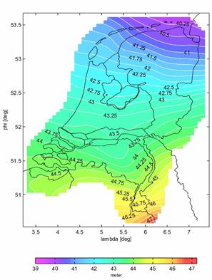
Figure 79 (left) comparison
of the local elevation datum in
12.1.2
Geographic
and square coordinates
Every
location on a geodetic datum is defined with a longitude angle and a latitude
angle of the ellipsoid. The fundamental point is the reference of these
angels. E.g. for WGS94 this is the
meridian of
The same
geographical coordinates of different datums will point in general to different
physical locations.
To make a
two dimensional map, the relevant part of the earth surface can be projected
onto a two dimensional plane. There are two conformal projection methods: A
projection onto a cone (called a Lambert Projection, see Figure 80) and a projection onto a cylinder (called a Mercator
projection, see Figure 81 ).
Figure 80 Lambert Projection:
a cone used to project the earth surface on. The map shows the developed red
part of the cone envelope. The
projection errors are negligible if only the projection is taken around the
contact region between the datum and the cone.
Figure 81 Mercator
projection: a cylinder used to project the earth surface on. The green map
shows the developed black squared part of the cylinder envelope. The projection
errors are negligible if only the projection is taken around the contact region
between the datum and the cylinder. Since the axis of revolution of the
cylinder is orthogonal to the rotation axis of the earth, this projection is
called a Transverse Mercator
projection.
(A conformal projection means that the scale in
one point is indifferent to the direction. This means that directions or angles
in the projected plane do correspond with the true angles that occur on the
datum surface. This can be important for navigation purposes where correct
directions over big distances is important)
In both projection planes, a location of a specific
point can be defined with planar or
square coordinates (observe the thick black lines on the maps): These
coordinates are called ‘Easting’ and ‘Northing’. Because of its visual aspect on a printed map
this is also called grid coordinates.
Some examples of local square coordinate systems:
o
In
Also, UTM
is used as coordinate system for the printed maps with datum ED50, and digital
maps with datum WGS84.
o
In
The Netherlands the datum RD 1918 is projected (oblique stereographic) locally
on a tangent plane. The corresponding square coordinate system is called Rijksdriehoekstelsel/Royal Dutch grid (Dutch grid).
Also, UTM
is used as coordinate system for the maps with datum WGS84.
To depict the whole earth on a map, multiple
successive projections of the entire datum can be made (polyconic or
polycylindric developments). Only the polycylindric development remains
conformal.
The Universal
Transverse Mercator projection (UTM)
is defined as of having 60 of such cylinders. They all project 360°/60=6° of
the datum along meridians.
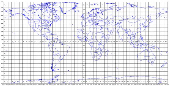
Figure 82 Universal Transverse Mercator projection. The Easting (longitudinal
zones) contains 60 projected zones (from 1 to 60), the Northing (latitudinal
zones) contains 20 zones (from C to X, I and 0 not used). Source http://www.dmap.co.uk/utmworld.htm
UTM coordinates look like this:
|
31 |
U |
603744 |
5648208 |
|
UTM time zone |
UTM band |
longitude in meters (Easting) |
latitude in meters (Northing) |
Table 8 UTM format
|
Summary: Cartographic maps have beside
its scale, two important properties: 1.
a specific datum,
2.
And a coordinate
system to be able to allocate each point on earth from this map. There are two coordinate
systems around: 1.
geographical
coordinates used on the datum spheroid: longitude and latitude angles 2.
square (or grid) coordinates used on a plane
projection: easting and northing The map compilation notes
always contain the scale, the chosen datum, the projection method when
applied, and the coordinate system. |
An
example:
The
following map uses geographical coordinates as well as two planar coordinate
systems:
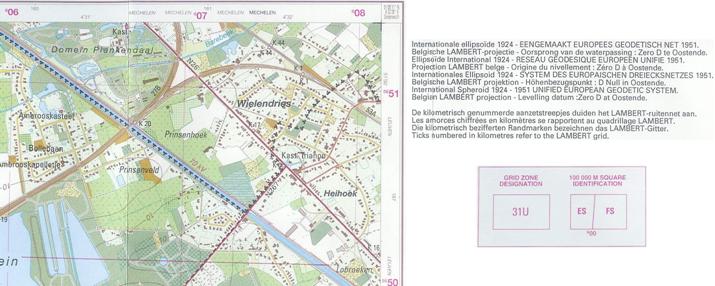
Figure 83 A topographical map
in  . The
other map compilation notes (see at the top right) show the used geodetic datum
(1951 Unified European Geodetic Datum = ED 50), used local geoid reference for levelling
data (Zero D at
. The
other map compilation notes (see at the top right) show the used geodetic datum
(1951 Unified European Geodetic Datum = ED 50), used local geoid reference for levelling
data (Zero D at
Remark that
the UTM grid lines are shown on a map with ED50 datum (which is another datum
as WGS84) and Lambert72 projection (which is not Transverse Mercator). Both
projection methods are conformal (preserve directions), so that might be the
reason why this is allowed.
Another
example shows a topo map of The Netherlands. Also here geographical coordinates
appear as well as two planar coordinates:
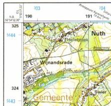
Figure 84 A topographical map
in The
12.2 GPS and maps
Each GPS
satellite transmits at the same instant data like their own location and the
current time. These signals move at the speed of light and arrive at the X9i.
Because the distance between each satellite and X9i differs, these signals arrive
at slightly different times. When the
receiver estimates at the same time the distance to at least four GPS
satellites, it can calculate its current position in three dimensions.
There are at least 24 operational GPS
satellites at all times. The satellites, operated by the U.S. Air Force, orbit
with a period of 12 hours. These satellites use WGS84 datum which also has a
center of gravity that matches with the true center of earth.
GPS receivers generate their position coordinates in general as longitude and latitude angles in a WGS84 datum. To compare a current location on the GPS display with the coordinates on a printed map, the GPS receiver is to be set with the same map datum and coordinate system. That way, the receiver makes the necessary calculations to display the coordinates in the same format as is done on the printed map.
A
different geodetic datum can cause errors up to hundreds of meters between the
displayed position and the correct position coordinates on a printed map. See Section 12.3.
A
different coordinate system (e.g. a global grid is used instead of a local grid)
disrupts in general every resemblance with the correct position coordinates on
a printed map.
If one is not interested in the instant displaying of the position coordinates, then it is in general not necessary to bother the datum and coordinate system in the GPS receiver.
12.3
Do
certain UTM coordinates refer always to the same location on earth?
A lot of
people think that a set of UTM coordinates (easting, northing) always refer to
the same location on earth, independent of the datum used. Similarly, one might
think that a set of geometrical coordinates (longitude and latitude) point to
the same location on earth.
To show
visually that this is a wrong assumption, I calibrated correctly a scanned topographic
map of a part of
|
31 |
U |
597691 |
5648536 |
|
UTM time zone |
UTM band |
longitude in meters (Easting) |
latitude in meters (Northing) |
Then I
switched the map DATUM to WGS84, and add another waypoint, but now by using the
previous UTM coordinates found.
Similarly,
I found the geographical coordinates of the bridge in the original ED50 DATUM:
|
4° 23.493’ E |
50° 58.745’ N |
|
longitude in degrees, decimal
minutes (Easting) |
latitude in degrees, decimal
minutes (Northing) |
Then I
added a third waypoint with the same longitude and latitude numbers, but now by
using the WGS84 DATUM. The results are shown in Figure
85 (I used
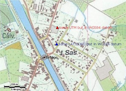
Figure 85 A bridge to far: The same UTM coordinates or LAT/LONG geographical coordinates refer to different positions on earth. To have a unique match, the correct map datum has to be known.
Conclusion: UTM coordinates (or longitude and
latitude geographical coordinates) as such are insufficient to trace the
correct position on a map: one always has to interpret the used coordinates
with regard to the used map DATUM. Coordinates alone are insufficient to define
a specific point on earth.
12.4 Further readings
|
Voor het Nederlands sprekend publiek in België en Nederland verwijs ik
graag naar twee excellente sites waar de basisbegirippen van geodesie, cartografie,
GPS en GPS navigatie eenvouding
uitgelegd worden. Een aanrader voor mensen die een eerste maal in
contact komen met GPS technologieen: Ø http://www.ngi.be/Common/articles/G/navigeren_met_GPS.pdf en http://www.ngi.be/NL/NL2-1-1.shtm
(net links naar basisbegrippen, coordinatensystemen, kaartvoorstellingen,
referentiesystemen) : een echte aanrader! Ø http://www.biodiv.nl/gps/ en http://www.ncg.knaw.nl/Publicaties/Groen/30Strang.html#Samenvatting
(met pdf link): nuttig voor de specifieke Nederlandse situatie. De relatie
tussen de world datums ETRS89 en WGS84
wordt eveneens uitgelegd. |
For the
English speaking people I refer as well to a general site on the working
principles of GPS; and a very fine course on geodesy, cartography and map
reading:
Ø
http://www.gmat.unsw.edu.au/snap/gps/gps_survey/principles_gps.htm
Ø
http://www.warnercnr.colostate.edu/class_info/nr502/mainpage/course_mainpage.html
Ø
If
you want to now more about the grids and datum’s used in your country, then you
will probably find the history of it in http://www.asprs.org/resources/grids/
. Some examples:
o
http://www.asprs.org/resources/grids/10-98-belgum.pdf on historical perspectives on the Belgian Datum
(BD72), Belgian Grid (Lambert72) and Elevation Datum (Zero D)
o
http://www.asprs.org/resources/grids/02-2003-netherlands.pdf on historical perspectives of the Dutch Datum
(RD1918), Dutch Grid (RD), and Elevation Datum (NAP). Relations between the
datums RD1918, ED50 and WGS84, and between the elevation datums AP, NAP and NN
are given as well.
Ø
http://www.asprs.org/resources/grids/04-2000-basic_datums.pdf
on the basics of classical datums.
STM has two
file formats:
1. a WaypointPlus file (ASCII
formatted, extension .txt) that only contains the time stamps
and position coordinates of a track, route or individual waypoint
2. a SuuntoDataFile (as well ASCII
formatted, extension .sdf) that contains also various other
data like altitudes for each track point or waypoint (if available), as well as
the recorded altitude log as is defined in
Table 5 of Section 4.1.1.
SUUNTO has sent me a shortened and public version of the sdf file format. You can download it from this location: http://www.wmin.be/sport/X9i/Suunto/Public%20version%20of%20sdf%20file%20description.doc
I feel
there is no need to work on these export files, since Olav Klein already did
the job perfectly (See Section 5.2).
This is a
must-know table for every X9i user.
|
key
press |
In DISPLAY |
behavior |
|
STOP/BACK |
TIME |
Change of parameter in lower line (dual time, stopwatch, seconds of time). It also stops the stopwatch when the stopwatch is running and on display. |
|
ALTI/BARO |
Change of parameter in lower line(time, temperature, absolute pressure) |
|
|
COMPASS |
Change of parameter in lower line(time, bearing lock ,bearing) |
|
|
ACTIVITY |
Change of parameter in lower line(time, time from start , altitude) |
|
|
START/DATA |
TIME |
Stopwatch Start/Lap when lower line shows the stopwatch |
|
ALTI/BARO |
Additional display showing time of sun rise and time of sun set of the day |
|
|
COMPASS when compass is not active |
Reactivate for 45 sec the compass (when ‘Start Compass’ was on the display) |
|
|
COMPASS when compass is active |
To create a Bearing fix of the current compass direction |
|
|
NAVIGATION |
Additional navigation data of the active Route |
|
|
ACTIVITY |
Additional activity data of the current Track log |
|
|
Long press STOP/BACK |
all |
Backlight on, if set to normal |
|
Long press START/DATA |
TIME |
Reset stopwatch if the lower line shows the stopwatch |
|
NAVIGATION + ACTIVITY |
When GPS is in PAUZE (GPSFIX 1min or manual), the GPS will be re-activated to take a track log sample and to update both displays. GPS returns thereafter to the current selected GPSFIX. |
(Internet
Explorer 5 and higher):
1. select the pull down menu
<File>;
2. Select the subfunction<Page
Setup…>;
3. In the Page Setup popup window,
select the encircled values. With these
setting you will obtain a correct copy (no cut off of the images and tables) of
the document.
With this, you can print the document directly on your printer.
To obtain an optimal print quality you can use as well the freware Cutepdf http://www.cutepdf.com/ ) or pdfCreator (http://www.pdfforge.org/products/pdfcreator ). This tool installs a virtual printer driver to which you can print this document to:
This virtual pdf printing creates a small sized quality pdf file of this compendium, which you can print from a Acrobat Reader or another pdf reader, or which you can save on your hard disk for later personal reading on your computer.